Note
Go to the end to download the full example code.
Training an FNO with incremental meta-learning
In this example, we demonstrate how to use the small Darcy-Flow example we ship with the package to demonstrate the Incremental FNO meta-learning algorithm
import torch
import matplotlib.pyplot as plt
import sys
from neuralop.models import FNO
from neuralop.data.datasets import load_darcy_flow_small
from neuralop.utils import count_model_params
from neuralop.training import AdamW
from neuralop.training.incremental import IncrementalFNOTrainer
from neuralop.data.transforms.data_processors import IncrementalDataProcessor
from neuralop import LpLoss, H1Loss
Loading the Darcy flow dataset
train_loader, test_loaders, output_encoder = load_darcy_flow_small(
    n_train=100,
    batch_size=16,
    test_resolutions=[16, 32],
    n_tests=[100, 50],
    test_batch_sizes=[32, 32],
)
/home/runner/work/neuraloperator/neuraloperator/neuralop/data/datasets/pt_dataset.py:93: FutureWarning: You are using `torch.load` with `weights_only=False` (the current default value), which uses the default pickle module implicitly. It is possible to construct malicious pickle data which will execute arbitrary code during unpickling (See https://github.com/pytorch/pytorch/blob/main/SECURITY.md#untrusted-models for more details). In a future release, the default value for `weights_only` will be flipped to `True`. This limits the functions that could be executed during unpickling. Arbitrary objects will no longer be allowed to be loaded via this mode unless they are explicitly allowlisted by the user via `torch.serialization.add_safe_globals`. We recommend you start setting `weights_only=True` for any use case where you don't have full control of the loaded file. Please open an issue on GitHub for any issues related to this experimental feature.
  data = torch.load(
Loading test db for resolution 16 with 100 samples
/home/runner/work/neuraloperator/neuraloperator/neuralop/data/datasets/pt_dataset.py:172: FutureWarning: You are using `torch.load` with `weights_only=False` (the current default value), which uses the default pickle module implicitly. It is possible to construct malicious pickle data which will execute arbitrary code during unpickling (See https://github.com/pytorch/pytorch/blob/main/SECURITY.md#untrusted-models for more details). In a future release, the default value for `weights_only` will be flipped to `True`. This limits the functions that could be executed during unpickling. Arbitrary objects will no longer be allowed to be loaded via this mode unless they are explicitly allowlisted by the user via `torch.serialization.add_safe_globals`. We recommend you start setting `weights_only=True` for any use case where you don't have full control of the loaded file. Please open an issue on GitHub for any issues related to this experimental feature.
  data = torch.load(Path(root_dir).joinpath(f"{dataset_name}_test_{res}.pt").as_posix())
Loading test db for resolution 32 with 50 samples
Choose device
device = torch.device("cuda" if torch.cuda.is_available() else "cpu")
Set up the incremental FNO model We start with 2 modes in each dimension We choose to update the modes by the incremental gradient explained algorithm
incremental = True
if incremental:
    starting_modes = (2, 2)
else:
    starting_modes = (16, 16)
set up model
model = FNO(
    max_n_modes=(16, 16),
    n_modes=starting_modes,
    hidden_channels=32,
    in_channels=1,
    out_channels=1,
)
model = model.to(device)
n_params = count_model_params(model)
Set up the optimizer and scheduler
optimizer = AdamW(model.parameters(), lr=8e-3, weight_decay=1e-4)
scheduler = torch.optim.lr_scheduler.CosineAnnealingLR(optimizer, T_max=30)


# If one wants to use Incremental Resolution, one should use the IncrementalDataProcessor - When passed to the trainer, the trainer will automatically update the resolution
# Incremental_resolution : bool, default is False
#    if True, increase the resolution of the input incrementally
#    uses the incremental_res_gap parameter
#    uses the subsampling_rates parameter - a list of resolutions to use
#    uses the dataset_indices parameter - a list of indices of the dataset to slice to regularize the input resolution
#    uses the dataset_resolution parameter - the resolution of the input
#    uses the epoch_gap parameter - the number of epochs to wait before increasing the resolution
#    uses the verbose parameter - if True, print the resolution and the number of modes
data_transform = IncrementalDataProcessor(
    in_normalizer=None,
    out_normalizer=None,
    device=device,
    subsampling_rates=[2, 1],
    dataset_resolution=16,
    dataset_indices=[2, 3],
    epoch_gap=10,
    verbose=True,
)

data_transform = data_transform.to(device)
Original Incre Res: change index to 0
Original Incre Res: change sub to 2
Original Incre Res: change res to 8
Set up the losses
l2loss = LpLoss(d=2, p=2)
h1loss = H1Loss(d=2)
train_loss = h1loss
eval_losses = {"h1": h1loss, "l2": l2loss}
print("\n### N PARAMS ###\n", n_params)
print("\n### OPTIMIZER ###\n", optimizer)
print("\n### SCHEDULER ###\n", scheduler)
print("\n### LOSSES ###")
print("\n### INCREMENTAL RESOLUTION + GRADIENT EXPLAINED ###")
print(f"\n * Train: {train_loss}")
print(f"\n * Test: {eval_losses}")
sys.stdout.flush()
### N PARAMS ###
 2110305

### OPTIMIZER ###
 AdamW (
Parameter Group 0
    betas: (0.9, 0.999)
    correct_bias: True
    eps: 1e-06
    initial_lr: 0.008
    lr: 0.008
    weight_decay: 0.0001
)

### SCHEDULER ###
 <torch.optim.lr_scheduler.CosineAnnealingLR object at 0x7fb4d68f2fd0>

### LOSSES ###

### INCREMENTAL RESOLUTION + GRADIENT EXPLAINED ###

 * Train: <neuralop.losses.data_losses.H1Loss object at 0x7fb4d573b750>

 * Test: {'h1': <neuralop.losses.data_losses.H1Loss object at 0x7fb4d573b750>, 'l2': <neuralop.losses.data_losses.LpLoss object at 0x7fb4d68f3490>}
Set up the IncrementalTrainer other options include setting incremental_loss_gap = True If one wants to use incremental resolution set it to True In this example we only update the modes and not the resolution When using the incremental resolution one should keep in mind that the numnber of modes initially set should be strictly less than the resolution Again these are the various paramaters for the various incremental settings incremental_grad : bool, default is False
if True, use the base incremental algorithm which is based on gradient variance uses the incremental_grad_eps parameter - set the threshold for gradient variance uses the incremental_buffer paramater - sets the number of buffer modes to calculate the gradient variance uses the incremental_max_iter parameter - sets the initial number of iterations uses the incremental_grad_max_iter parameter - sets the maximum number of iterations to accumulate the gradients
- incremental_loss_gapbool, default is False
if True, use the incremental algorithm based on loss gap uses the incremental_loss_eps parameter
# Finally pass all of these to the Trainer
trainer = IncrementalFNOTrainer(
    model=model,
    n_epochs=20,
    data_processor=data_transform,
    device=device,
    verbose=True,
    incremental_loss_gap=False,
    incremental_grad=True,
    incremental_grad_eps=0.9999,
    incremental_loss_eps = 0.001,
    incremental_buffer=5,
    incremental_max_iter=1,
    incremental_grad_max_iter=2,
)
Train the model
trainer.train(
    train_loader,
    test_loaders,
    optimizer,
    scheduler,
    regularizer=False,
    training_loss=train_loss,
    eval_losses=eval_losses,
)
Training on 100 samples
Testing on [50, 50] samples         on resolutions [16, 32].
Raw outputs of shape torch.Size([16, 1, 8, 8])
[0] time=0.24, avg_loss=0.9239, train_err=13.1989
Eval: 16_h1=0.8702, 16_l2=0.5536, 32_h1=0.9397, 32_l2=0.5586
[1] time=0.22, avg_loss=0.7589, train_err=10.8413
Eval: 16_h1=0.7880, 16_l2=0.5167, 32_h1=0.9011, 32_l2=0.5234
[2] time=0.23, avg_loss=0.6684, train_err=9.5484
Eval: 16_h1=0.7698, 16_l2=0.4235, 32_h1=0.9175, 32_l2=0.4405
[3] time=0.22, avg_loss=0.6082, train_err=8.6886
Eval: 16_h1=0.7600, 16_l2=0.4570, 32_h1=1.0126, 32_l2=0.5005
[4] time=0.22, avg_loss=0.5604, train_err=8.0054
Eval: 16_h1=0.8301, 16_l2=0.4577, 32_h1=1.1722, 32_l2=0.4987
[5] time=0.23, avg_loss=0.5366, train_err=7.6663
Eval: 16_h1=0.8099, 16_l2=0.4076, 32_h1=1.1414, 32_l2=0.4436
[6] time=0.23, avg_loss=0.5050, train_err=7.2139
Eval: 16_h1=0.7204, 16_l2=0.3888, 32_h1=0.9945, 32_l2=0.4285
[7] time=0.23, avg_loss=0.4429, train_err=6.3271
Eval: 16_h1=0.6197, 16_l2=0.3479, 32_h1=0.8862, 32_l2=0.3924
[8] time=0.23, avg_loss=0.4058, train_err=5.7968
Eval: 16_h1=0.6224, 16_l2=0.3372, 32_h1=0.8627, 32_l2=0.3706
[9] time=0.23, avg_loss=0.3775, train_err=5.3930
Eval: 16_h1=0.5841, 16_l2=0.3159, 32_h1=0.8551, 32_l2=0.3587
Incre Res Update: change index to 1
Incre Res Update: change sub to 1
Incre Res Update: change res to 16
[10] time=0.28, avg_loss=0.5158, train_err=7.3681
Eval: 16_h1=0.5133, 16_l2=0.3167, 32_h1=0.6120, 32_l2=0.3022
[11] time=0.27, avg_loss=0.4536, train_err=6.4795
Eval: 16_h1=0.4680, 16_l2=0.3422, 32_h1=0.6436, 32_l2=0.3659
[12] time=0.28, avg_loss=0.4155, train_err=5.9358
Eval: 16_h1=0.4119, 16_l2=0.2692, 32_h1=0.5285, 32_l2=0.2692
[13] time=0.28, avg_loss=0.3724, train_err=5.3195
Eval: 16_h1=0.4045, 16_l2=0.2569, 32_h1=0.5620, 32_l2=0.2747
[14] time=0.28, avg_loss=0.3555, train_err=5.0783
Eval: 16_h1=0.3946, 16_l2=0.2485, 32_h1=0.5278, 32_l2=0.2523
[15] time=0.28, avg_loss=0.3430, train_err=4.8998
Eval: 16_h1=0.3611, 16_l2=0.2323, 32_h1=0.5079, 32_l2=0.2455
[16] time=0.28, avg_loss=0.3251, train_err=4.6438
Eval: 16_h1=0.3433, 16_l2=0.2224, 32_h1=0.4757, 32_l2=0.2351
[17] time=0.28, avg_loss=0.3072, train_err=4.3888
Eval: 16_h1=0.3458, 16_l2=0.2226, 32_h1=0.4776, 32_l2=0.2371
[18] time=0.28, avg_loss=0.2982, train_err=4.2593
Eval: 16_h1=0.3251, 16_l2=0.2116, 32_h1=0.4519, 32_l2=0.2245
[19] time=0.28, avg_loss=0.2802, train_err=4.0024
Eval: 16_h1=0.3201, 16_l2=0.2110, 32_h1=0.4533, 32_l2=0.2245

{'train_err': 4.002395851271493, 'avg_loss': 0.2801677095890045, 'avg_lasso_loss': None, 'epoch_train_time': 0.28232425900000635, '16_h1': tensor(0.3201), '16_l2': tensor(0.2110), '32_h1': tensor(0.4533), '32_l2': tensor(0.2245)}
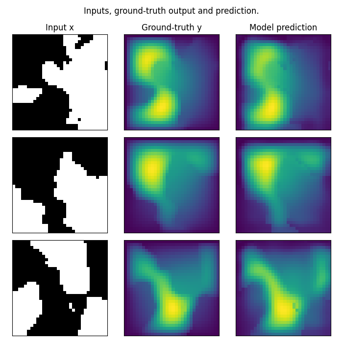
Plot the prediction, and compare with the ground-truth Note that we trained on a very small resolution for a very small number of epochs In practice, we would train at larger resolution, on many more samples.
However, for practicity, we created a minimal example that i) fits in just a few Mb of memory ii) can be trained quickly on CPU
In practice we would train a Neural Operator on one or multiple GPUs
test_samples = test_loaders[32].dataset

fig = plt.figure(figsize=(7, 7))
for index in range(3):
    data = test_samples[index]
    # Input x
    x = data["x"].to(device)
    # Ground-truth
    y = data["y"].to(device)
    # Model prediction
    out = model(x.unsqueeze(0))
    ax = fig.add_subplot(3, 3, index * 3 + 1)
    x = x.cpu().squeeze().detach().numpy()
    y = y.cpu().squeeze().detach().numpy()
    ax.imshow(x, cmap="gray")
    if index == 0:
        ax.set_title("Input x")
    plt.xticks([], [])
    plt.yticks([], [])

    ax = fig.add_subplot(3, 3, index * 3 + 2)
    ax.imshow(y.squeeze())
    if index == 0:
        ax.set_title("Ground-truth y")
    plt.xticks([], [])
    plt.yticks([], [])

    ax = fig.add_subplot(3, 3, index * 3 + 3)
    ax.imshow(out.cpu().squeeze().detach().numpy())
    if index == 0:
        ax.set_title("Model prediction")
    plt.xticks([], [])
    plt.yticks([], [])

fig.suptitle("Inputs, ground-truth output and prediction.", y=0.98)
plt.tight_layout()
fig.show()
Total running time of the script: (0 minutes 6.988 seconds)