Note
Go to the end to download the full example code.
Divergence-Free Spectral Projection
An example demonstrating spectral projection to enforce divergence-free constraints in 2D velocity fields
Import the library
We first import our neuralop library and required dependencies.
import torch
import numpy as np
import matplotlib.pyplot as plt
from neuralop.layers.spectral_projection import spectral_projection_divergence_free
from neuralop.losses.differentiation import FourierDiff, FiniteDiff

device = torch.device("cuda" if torch.cuda.is_available() else "cpu")
print(f"Using device: {device}")
Using device: cpu
Divergence error computation functions
We define two functions to compute the divergence error using spectral differentiation and finite differences.
def div_error_fourier(u, L):
    """Compute divergence error using spectral differentiation."""
    fourier_diff_2d = FourierDiff(dim=2, L=(L, L), use_fc=False)
    div = fourier_diff_2d.divergence(u)
    error_val = torch.linalg.norm(div, dim=(1, 2)) * (L**2 / (div.shape[-1] * div.shape[-2]))**(0.5)
    return error_val.mean().item()


def div_error_finite_diff(u, L):
    """Compute divergence error using FiniteDiff."""
    dx = L / u.shape[-1]
    dy = L / u.shape[-2]
    finite_diff_2d = FiniteDiff(dim=2, h=(dx, dy), periodic_in_x=True, periodic_in_y=True)
    div = finite_diff_2d.divergence(u)
    error_val = torch.linalg.norm(div, dim=(1, 2)) * (L**2 / (div.shape[-1] * div.shape[-2]))**(0.5)
    return error_val.mean().item()
Setting considered
We start from a divergence-free velocity field on [0, 2*pi] x [0, 2*pi] constructed from the stream function ψ(x,y) = sin(x) * cos(6*y)
- Velocity components:
u_x = ∂ψ/∂y = -6 * sin(x) * sin(6*y)
u_y = -∂ψ/∂x = - cos(x) * cos(6*y)
Mathematical verification of divergence-free property:
∇·u = ∂u_x/∂x + ∂u_y/∂y
= ∂/∂x[-6*sin(x) * sin(6*y)] + ∂/∂y[-cos(x) * cos(6*y)]
= -6*cos(x) * sin(6*y) + 6*cos(x) * sin(6*y)
= 0 ✓
We then add 10% noise to break the divergence-free property.
We then apply the spectral projection to restore the divergence-free property.
We then compute the divergence error for the original, noisy, and projected fields.
We repeat this at various resolutions, [256, 512, 1024, 2048, 4096, 8192].
L = 2 * np.pi
noise_level = 0.1
resolutions = [256, 512, 1024, 2048, 4096, 8192]


errors_original_spectral = []
errors_original_finite = []
errors_noisy_spectral = []
errors_noisy_finite = []
errors_prog_spectral = []
errors_prog_finite = []

for target_resolution in resolutions:
    # Create coordinate grids for this resolution
    xs = torch.arange(target_resolution, device=device, dtype=torch.float64) * (L / target_resolution)
    ys = torch.arange(target_resolution, device=device, dtype=torch.float64) * (L / target_resolution)
    X, Y = torch.meshgrid(xs, ys, indexing="ij")

    # Create divergence-free field using the stream function defined earlier
    u_x = -6.0 * torch.sin(X) * torch.sin(6.0 * Y)
    u_y = -torch.cos(X) * torch.cos(6.0 * Y)
    u = torch.stack([u_x, u_y], dim=0).unsqueeze(0).to(device=device, dtype=torch.float64)

    # Add noise to break divergence-free property
    mean_magnitude = torch.mean(torch.sqrt(u[:, 0] ** 2 + u[:, 1] ** 2))
    noise = torch.randn_like(u, dtype=torch.float64) * noise_level * mean_magnitude
    u_noisy = u + noise

    # Apply spectral projection to restore divergence-free property
    u_proj = spectral_projection_divergence_free(u_noisy, L, constraint_modes=(64, 64))

    # Compute divergence errors for all three fields
    errors_original_spectral.append(div_error_fourier(u, L))
    errors_original_finite.append(div_error_finite_diff(u, L))
    errors_noisy_spectral.append(div_error_fourier(u_noisy, L))
    errors_noisy_finite.append(div_error_finite_diff(u_noisy, L))
    errors_prog_spectral.append(div_error_fourier(u_proj, L))
    errors_prog_finite.append(div_error_finite_diff(u_proj, L))
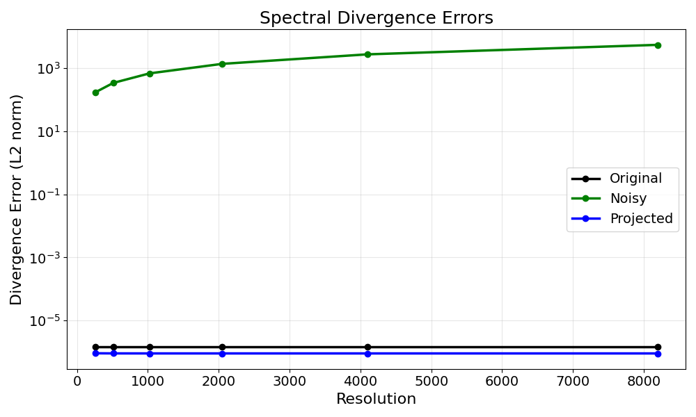
Divergence Errors using Spectral Differentiation
The Fourier differentiation method computes derivatives in the spectral domain by transforming the field to Fourier space, applying the appropriate wavenumber operators, and transforming back.
We display the divergence error for the original, noisy, and projected fields at the different resolutions.
Note that at lower resolutions, finite differences are not accurate enough to properly compute the divergence error, which is why the errors appear higher initially but improve at higher resolutions. This is a limitation of finite differences for computing derivatives, not an issue with the spectral projection itself. Spectral differentiation provides more accurate derivative calculations at lower resolutions.
# Spectral Differentiation table
print("-" * 55)
print(f"{'Resolution':<12} {'Original':<15} {'Noisy':<15} {'Projected':<15}")
print("-" * 55)

for i, res in enumerate(resolutions):
    print(
        f"{res:<12} {errors_original_spectral[i]:<15.2e} {errors_noisy_spectral[i]:<15.2e} {errors_prog_spectral[i]:<15.2e}"
    )


# Spectral Differentiation plot
plt.figure(figsize=(10, 6))
plt.semilogy(resolutions, errors_original_spectral, "o-", label="Original", color="black", linewidth=2.5, markersize=6)
plt.semilogy(resolutions, errors_noisy_spectral, "o-", label="Noisy", color="green", linewidth=2.5, markersize=6)
plt.semilogy(resolutions, errors_prog_spectral, "o-", label="Projected", color="blue", linewidth=2.5, markersize=6)
plt.xlabel("Resolution", fontsize=16)
plt.ylabel("Divergence Error (L2 norm)", fontsize=16)
plt.title("Spectral Divergence Errors", fontsize=18)
plt.legend(fontsize=14)
plt.grid(True, alpha=0.3)
plt.xticks(fontsize=14)
plt.yticks(fontsize=14)
plt.tight_layout()
plt.show()
-------------------------------------------------------
Resolution   Original        Noisy           Projected
-------------------------------------------------------
256          1.50e-06        1.69e+02        9.20e-07
512          1.50e-06        3.37e+02        9.12e-07
1024         1.50e-06        6.77e+02        9.10e-07
2048         1.50e-06        1.35e+03        9.10e-07
4096         1.50e-06        2.71e+03        9.10e-07
8192         1.50e-06        5.42e+03        9.10e-07
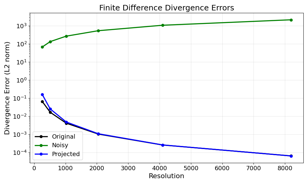
Divergence Errors using Finite Differences
The finite difference method approximates derivatives using central differences.
We display the divergence error for the original, noisy, and projected fields at the different resolutions.
# Finite differences table
print("-" * 55)
print(f"{'Resolution':<12} {'Original':<15} {'Noisy':<15} {'Projected':<15}")
print("-" * 55)

for i, res in enumerate(resolutions):
    print(
        f"{res:<12} {errors_original_finite[i]:<15.2e} {errors_noisy_finite[i]:<15.2e} {errors_prog_finite[i]:<15.2e}"
    )


# Finite differences plot
plt.figure(figsize=(10, 6))
plt.semilogy(resolutions, errors_original_finite, "o-", label="Original", color="black", linewidth=2.5, markersize=6)
plt.semilogy(resolutions, errors_noisy_finite, "o-", label="Noisy", color="green", linewidth=2.5, markersize=6)
plt.semilogy(resolutions, errors_prog_finite, "o-", label="Projected", color="blue", linewidth=2.5, markersize=6)
plt.xlabel("Resolution", fontsize=16)
plt.ylabel("Divergence Error (L2 norm)", fontsize=16)
plt.title("Finite Difference Divergence Errors", fontsize=18)
plt.legend(fontsize=14)
plt.grid(True, alpha=0.3)
plt.xticks(fontsize=14)
plt.yticks(fontsize=14)
plt.tight_layout()
plt.show()
-------------------------------------------------------
Resolution   Original        Noisy           Projected
-------------------------------------------------------
256          6.62e-02        6.61e+01        1.62e-01
512          1.66e-02        1.32e+02        2.53e-02
1024         4.14e-03        2.64e+02        4.81e-03
2048         1.03e-03        5.28e+02        1.08e-03
4096         2.59e-04        1.06e+03        2.61e-04
8192         6.47e-05        2.11e+03        6.43e-05
Total running time of the script: (0 minutes 39.471 seconds)