Resampling layers

When working with neural operators, we often need to change the resolution of our data. For some architectures, like the FNO, this is handled automatically due to the resolution-invariant nature of the Fourier domain.

However, for other architectures, like the U-Net, we need to explicitly upsample and downsample the data as it flows through the network. The neuralop.layers.resample function provides a convenient way to do this.

In this example, we’ll demonstrate how to use the resample function to upsample and downsample a sample from a Gaussian Random Field, which serves as a better visual tool than piecewise constant data for observing the effects of interpolation.

For 1D and 2D inputs, the resample function uses PyTorch’s built-in spatial interpolators for efficiency, applying linear interpolation for 1D data and bicubic interpolation for 2D data directly in the spatial domain.

For 3D or higher-dimensional inputs, the resample function switches to a spectral interpolation method based on the Fourier transform. The input is transformed into the frequency domain using a real n-dimensional FFT, which decomposes the signal into its frequency components. By resizing this frequency representation and then applying an inverse FFT, the function achieves smooth, alias-free interpolation that preserves the signal’s overall structure.

import torch
import matplotlib.pyplot as plt
from neuralop.layers.resample import resample

First, let’s generate a data input. We create a high-resolution Gaussian Random Field (GRF), which is a smooth, continuous signal, making it ideal for visualizing the effects of resampling.

device = "cpu"


def generate_grf(shape, alpha=2.5, device="cpu"):
    """Generates a 2D Gaussian Random Field.

    Parameters
    ----------
    shape : tuple
        The desired output shape (height, width).
    alpha : float, optional
        A parameter controlling the smoothness of the field.
        Higher alpha leads to smoother fields, by default 2.5.
    device : str, optional
        The device to create the tensor on, by default 'cpu'.

    Returns
    -------
    torch.Tensor
        A 4D tensor of shape (1, 1, height, width) containing the GRF.
    """
    n, m = shape
    freq_x = torch.fft.fftfreq(n, d=1 / n, device=device).view(-1, 1)
    freq_y = torch.fft.fftfreq(m, d=1 / m, device=device).view(1, -1)

    norm_sq = freq_x**2 + freq_y**2
    norm_sq[0, 0] = 1.0  # Avoid division by zero

    # Generate white noise in frequency domain
    noise = torch.randn(n, m, dtype=torch.cfloat, device=device)

    # Apply a power-law filter
    filtered_noise = noise * (norm_sq ** (-alpha / 2.0))

    # Inverse FFT to get the spatial field
    field = torch.fft.ifft2(filtered_noise).real

    # Normalize to [0, 1] for visualization
    field = (field - field.min()) / (field.max() - field.min())

    return field.unsqueeze(0).unsqueeze(0)  # Add batch and channel dims


# Generate a 128x128 sample as our ground truth
high_res = 128
high_res_data = generate_grf((high_res, high_res), device=device)

# Define the low resolution we want to simulate (4x downsampling)
low_res = 32

Now, let’s use the resample function to simulate downsampling and upsampling operations. This could for instance be used in the encoder and decoder of a U-Net architecture. The function takes an input tensor, a scale_factor, and a list of axis dimensions to which the resampling is applied.

# To downsample from 128x128 to 32x32, we need a scale factor of 32/128 = 0.25
downsample_factor = low_res / high_res
downsampled_data = resample(high_res_data, downsample_factor, [2, 3])

# To upsample from 32x32 back to 128x128, we need a scale factor of 128/32 = 4
upsample_factor = high_res / low_res
upsampled_data = resample(downsampled_data, upsample_factor, [2, 3])

Finally, let’s visualize the results to see the effect of the resample function.

fig, axs = plt.subplots(1, 3, figsize=(14, 6))
plt.subplots_adjust(wspace=0.04)
fig.suptitle("Resampling a Gaussian Random Field", fontsize=24)

# Plot the original high-resolution data
im1 = axs[0].imshow(high_res_data.squeeze().cpu().numpy(), cmap="viridis", vmin=0, vmax=1)
axs[0].set_title(f"High-Res Data ({high_res}x{high_res})", fontsize=16, fontweight="bold")
cbar1 = fig.colorbar(im1, ax=axs[0], fraction=0.046, pad=0.04, ticks=[0, 0.5, 1])
cbar1.ax.tick_params(labelsize=14)

# Plot the downsampled data
im2 = axs[1].imshow(downsampled_data.squeeze().cpu().numpy(), cmap="viridis", vmin=0, vmax=1)
axs[1].set_title(f"Downsampled (x{downsample_factor}) ({low_res}x{low_res})", fontsize=16, fontweight="bold")
cbar2 = fig.colorbar(im2, ax=axs[1], fraction=0.046, pad=0.04, ticks=[0, 0.5, 1])
cbar2.ax.tick_params(labelsize=14)

# Plot the upsampled data
im3 = axs[2].imshow(upsampled_data.squeeze().cpu().numpy(), cmap="viridis", vmin=0, vmax=1)
axs[2].set_title(f"Upsampled Back (x{upsample_factor:.0f}) ({high_res}x{high_res})", fontsize=16, fontweight="bold")
cbar3 = fig.colorbar(im3, ax=axs[2], fraction=0.046, pad=0.04, ticks=[0, 0.5, 1])
cbar3.ax.tick_params(labelsize=14)

# Hide axis ticks for a cleaner look
for ax in axs.flat:
    ax.set_xticks([])
    ax.set_yticks([])

plt.tight_layout(rect=[0, 0.03, 1, 1.08])
plt.show()

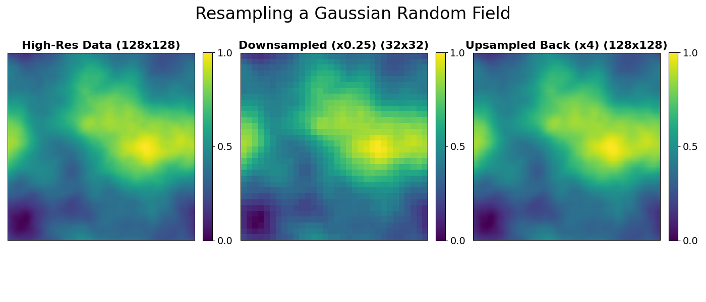
Resampling a Gaussian Random Field, High-Res Data (128x128), Downsampled (x0.25) (32x32), Upsampled Back (x4) (128x128)

The resample function effectively changes the resolution of the data. Notice that the upsampled image on the right is a faithful, if slightly blurrier, reconstruction of the original. This is because the downsampling step is lossy; high-frequency details are lost and cannot be perfectly recovered.

Total running time of the script: (0 minutes 0.272 seconds)

Gallery generated by Sphinx-Gallery