Note
Go to the end to download the full example code.
Grid Embeddings
Grid embeddings encode spatial coordinates in neural operators, helping models understand geometric structure. This tutorial shows how to use:
2D and N-dimensional grid embeddings
Custom coordinate systems
Different embedding types for various domains
Grid embeddings are key for PDE solving, computer vision, and other spatially-structured problems. They add coordinate information and help neural operators learn spatial relationships.
Import dependencies
We import the necessary modules for working with grid embeddings
import random
import matplotlib.pyplot as plt
import torch

device = "cpu"
Understanding grid embeddings
As we show in A simple Darcy-Flow dataset, we apply a 2D grid positional encoding to our data before passing it into the FNO. This embedding has been shown to improve model performance in a variety of applications by providing spatial context to the neural operator.
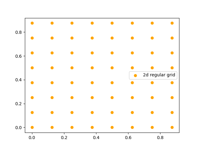
Let’s walk through its use. We start with a function that gives the coordinates of the bottom-left corners of each pixel in a grid:
from neuralop.layers.embeddings import regular_grid_2d

grid_2d = (
    torch.stack(regular_grid_2d(spatial_dims=(8, 8))).permute(1, 2, 0).view(-1, 2)
)  # reshape into (64, 2)

# Visualize the 2D grid coordinates
plt.scatter(grid_2d[:, 0], grid_2d[:, 1], color="orange", label="2D regular grid")
plt.legend()
plt.title("2D Grid Coordinates")
plt.xlabel("X coordinate")
plt.ylabel("Y coordinate")
plt.show()
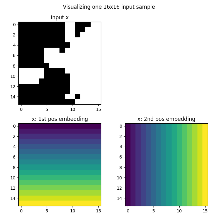
Applying grid embeddings to data
In practice, we concatenate these two channels, representing the x- and y-coordinates of each pixel in an example, after the channels which encode physical variables in our PDE problems. This provides spatial context to the neural operator.
from neuralop.data.datasets import load_darcy_flow_small
from neuralop.layers.embeddings import GridEmbedding2D

# Load the Darcy-Flow dataset for demonstration
_, test_loaders, _ = load_darcy_flow_small(
    n_train=10,
    batch_size=1,
    test_resolutions=[16, 32],
    n_tests=[16, 16],
    test_batch_sizes=[2, 2],
    encode_output=False,
)

# Get a sample from the dataset
loader_16 = test_loaders[16]
example = next(iter(loader_16))
x = example["x"]
print(f"One batch of x is of shape: {x.shape}")

# Note: our Darcy dataset is generated on the unit square, but our grid
# embedding's boundaries are configurable.
grid_embedding = GridEmbedding2D(in_channels=1, grid_boundaries=[[0, 1], [0, 1]])
x = grid_embedding(x)
print(f"After embedding, x is of shape: {x.shape}")
Loading test db for resolution 16 with 16 samples
Loading test db for resolution 32 with 16 samples
/opt/hostedtoolcache/Python/3.13.14/x64/lib/python3.13/site-packages/torch/utils/data/dataloader.py:1095: UserWarning: 'pin_memory' argument is set as true but no accelerator is found, then device pinned memory won't be used.
  super().__init__(loader)
One batch of x is of shape: torch.Size([2, 1, 16, 16])
After embedding, x is of shape: torch.Size([2, 3, 16, 16])
Visualizing the embedded data
We can visualize how the grid embedding adds coordinate information to our data. The embedding adds two channels: one for x-coordinates and one for y-coordinates.
# Grab the first element of the batch
x = x[0]
fig = plt.figure(figsize=(7, 7))

# Plot the original input data
ax = fig.add_subplot(2, 2, 1)
ax.imshow(x[0], cmap="gray")
ax.set_title("Input x")

# Plot the x-coordinate embedding
ax = fig.add_subplot(2, 2, 3)
ax.imshow(x[1])
ax.set_title("x-coordinate embedding")

# Plot the y-coordinate embedding
ax = fig.add_subplot(2, 2, 4)
ax.imshow(x[2])
ax.set_title("y-coordinate embedding")

fig.suptitle("Visualizing one input sample with positional embeddings", y=0.98)
plt.tight_layout()
fig.show()
Discretization invariance
Our embeddings are also designed with discretization-invariance in mind. Without any changes, we can apply the same embedding to higher-resolution data. This is crucial for neural operators that need to work at different resolutions.
loader_32 = test_loaders[32]
example = next(iter(loader_32))
x = example["x"]
print(f"One batch of x is of shape: {x.shape}")

# Apply the same grid embedding to higher-resolution data
x = grid_embedding(x)
print(f"After embedding, x is of shape: {x.shape}")
One batch of x is of shape: torch.Size([2, 1, 32, 32])
After embedding, x is of shape: torch.Size([2, 3, 32, 32])
Visualizing higher-resolution embeddings
We can see how the grid embedding scales to different resolutions. The coordinate information is automatically adjusted to the new grid size.
# Grab the first element of the batch
x = x[0]
fig = plt.figure(figsize=(7, 7))

# Plot the original input data
ax = fig.add_subplot(2, 2, 1)
ax.imshow(x[0], cmap="gray")
ax.set_title("Input x")

# Plot the x-coordinate embedding
ax = fig.add_subplot(2, 2, 3)
ax.imshow(x[1])
ax.set_title("x-coordinate embedding")

# Plot the y-coordinate embedding
ax = fig.add_subplot(2, 2, 4)
ax.imshow(x[2])
ax.set_title("y-coordinate embedding")

fig.suptitle("Visualizing one input sample with positional embeddings", y=0.98)
plt.tight_layout()
fig.show()
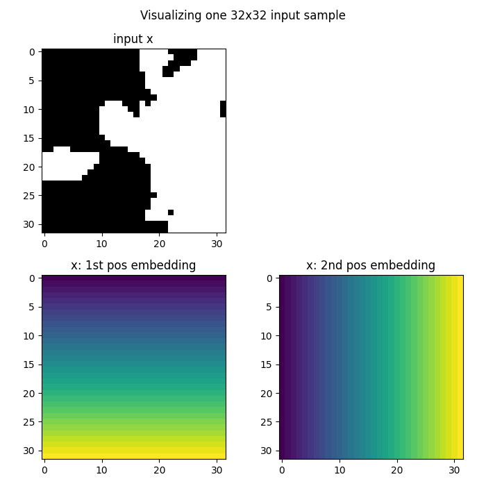
Understanding discretization invariance
The grid embeddings automatically adapt to different resolutions: 1. The coordinate values are normalized to the same range regardless of resolution 2. The spatial relationships are preserved across different grid sizes 3. This allows neural operators to work seamlessly at different resolutions 4. The same model can be applied to data of varying spatial discretization
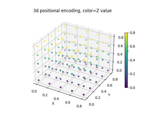
Working with 3D grid embeddings
Let’s also demonstrate how to embed a 3D tensor. This is useful for problems involving 3D spatial data, such as: - 3D fluid dynamics - Volumetric medical imaging - 3D material science problems
from neuralop.layers.embeddings import GridEmbeddingND

# Create a 3D tensor with one channel
cube_len = 5
x = torch.randn(1, 1, cube_len, cube_len, cube_len)
embedding_3d = GridEmbeddingND(in_channels=1, dim=3, grid_boundaries=[[0, 1]] * 3)

# Apply 3D grid embedding
x = embedding_3d(x)
Visualizing 3D grid embeddings
We can visualize the 3D embeddings by showing the coordinate information in 3D space. Each point represents a spatial location with its coordinates.
# Grab only the appended positional embedding channels
x = x[0, 1:, ...].permute(1, 2, 3, 0).view(-1, 3)
fig, ax = plt.subplots(subplot_kw={"projection": "3d"})
plot = ax.scatter(x[:, 0], x[:, 1], x[:, 2], c=x[:, 2])
fig.colorbar(plot, ax=ax, shrink=0.6)
ax.set_title("3D positional encoding, color=Z value")
ax.set_xlabel("X")
ax.set_ylabel("Y")
ax.set_zlabel("Z")
plt.show()
Total running time of the script: (0 minutes 0.728 seconds)