Neighbor Search for Graph Neural Operators

This tutorial demonstrates neighbor search algorithms used in Graph Neural Operators (GNO). Neighbor search is crucial for:

Finding spatial relationships in irregular point clouds
Computing Nyström approximations of kernel integrals
Enabling GNO to work with arbitrary point cloud data
Implementing efficient spatial queries for neural operators

The tutorial covers the native_neighbor_search function and its role in GNO architectures.

Import dependencies

We import the necessary modules for neighbor search and visualization

import random
import matplotlib.pyplot as plt
import torch

from neuralop.layers.gno_block import GNOBlock
from neuralop.layers.neighbor_search import native_neighbor_search
from neuralop.layers.embeddings import regular_grid_2d

device = "cpu"

Understanding Graph Neural Operators and neighbor search

Many problems involve data collected over irregular point clouds. The Graph Neural Operator (GNO) is a neural operator architecture that learns mappings between functions evaluated on arbitrary point clouds.

For input coordinates Y, input function f evaluated at all y ∈ Y, and output coordinates X, our goal is to map to function g evaluated at all x ∈ X. The GNO computes the Nyström approximation of a continuous kernel integral: ∫_{N_r(x)} f(y) k(x,y) dy

The first step is neighbor search to find spatial relationships.

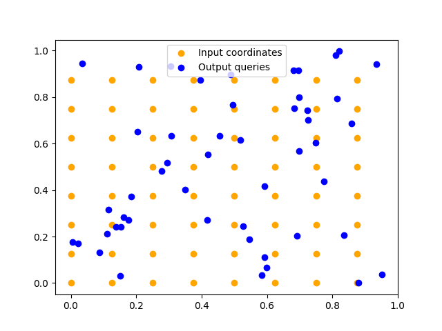
Setting up the point cloud data

We create a regular grid of input coordinates and random output query points to demonstrate the neighbor search functionality.

# Create a regular 8x8 grid of input coordinates
input_coords = (
    torch.stack(regular_grid_2d(spatial_dims=(8, 8))).permute(1, 2, 0).view(-1, 2)
)

# Generate random output query points
output_queries = torch.rand([50, 2])

# Visualize the input coordinates and query points
plt.scatter(
    input_coords[:, 0],
    input_coords[:, 1],
    color="orange",
    label="Input coordinates",
    s=50,
)
plt.scatter(
    output_queries[:, 0],
    output_queries[:, 1],
    color="blue",
    label="Output queries",
    s=30,
)
plt.legend()
plt.title("Input coordinates and output query points")
plt.xlabel("x")
plt.ylabel("y")
plt.show()

Input coordinates and output query points

Performing neighbor search

We select a query point and find all input coordinates within a specified radius. This demonstrates how the neighbor search algorithm identifies spatial relationships.

query_index = 6
query_point = output_queries[query_index]

# Perform neighbor search with radius 0.25
# Note: This radius is relatively large for our data density.
# In practice, we typically use values that find around 10 neighbors.
nbr_data = native_neighbor_search(
    data=input_coords, queries=query_point.unsqueeze(0), radius=0.25
)

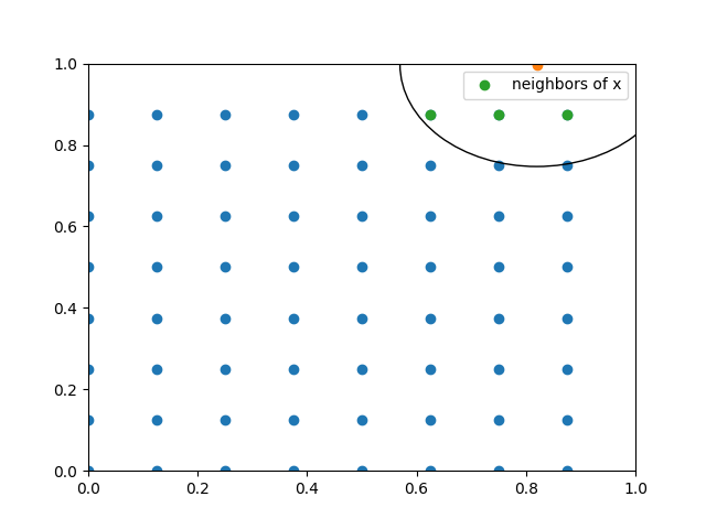
Visualizing the neighbor search results

We plot the query point, its neighbors, and the search radius to understand how the neighbor search algorithm works.

fig, ax = plt.subplots()
neighbors = input_coords[nbr_data["neighbors_index"]]
ax.scatter(
    input_coords[:, 0], input_coords[:, 1], color="blue", label="Input coordinates"
)
ax.scatter(
    query_point[0], query_point[1], color="red", marker="*", s=200, label="Query point"
)
ax.scatter(neighbors[:, 0], neighbors[:, 1], color="green", label="Neighbors of query")
c = plt.Circle(query_point, radius=0.25, fill=False)
ax.add_patch(c)

ax.legend()
ax.set_xlim(0, 1)
ax.set_ylim(0, 1)

(0.0, 1.0)

Total running time of the script: (0 minutes 0.144 seconds)

Gallery generated by Sphinx-Gallery