Note
Go to the end to download the full example code.
Sinusoidal Embeddings
Inputs to deep learning models often represent positions on a spatial, temporal, or spatio-temporal grid. To enrich these coordinates, positional embeddings can be introduced to improve a model’s capacity to generalize across the domain. In this tutorial, we focus on sinusoidal positional embeddings.
Sinusoidal embeddings encode inputs as periodic functions (sines and cosines), thereby lifting low-dimensional coordinates into a richer spectral representation. This spectral lifting enhances the model’s ability to capture fine-scale variations and high-frequency dynamics.
Setup in 1D
To build intuition, consider a simple 1D example. Let \(x \in \mathbb{R}\) be a single input, and define the embedding function
where \(L\) defines the number of frequencies we wish to use for the embedding. Each pair of sine and cosine terms introduces a higher frequency, enriching how positional information is represented.
This idea naturally extends to an entire 1D input. Let \(\vec{x} \in \mathbb{R}^N\) denote a discretized domain of \(N\) points. Then the embedding function becomes
In practice, both the original coordinate and its embedding are passed to the model:
preserving the original input, while augmenting it with a hierarchy of frequency components.
Domain Normalization
When applying sinusoidal embeddings, it is often useful to normalize the input coordinates to a periodic interval that aligns with the natural period of the sine and cosine functions. For example, a 1D spatial domain \(\vec{x} \in[0,1]\) of \(N\) points can be rescaled to
so that \(\vec{x}^{\prime} \in[0,2 \pi]\).
This mapping preserves the number of sampling points \(N\) and the overall shape of the domain while ensuring that the lowest-frequency sine and cosine components complete exactly one full oscillation over the interval.
Choosing \(L\) to Satisfy the Nyquist-Criterion
Warning
When choosing the number of frequency levels \(L\), it is important to ensure that the highest frequency component in the embedding does not exceed the Nyquist limit imposed by the discretisation of the input domain.
For a domain of \(N\) points, the Nyquist frequency is
For the sinusoidal embedding defined above, the Nyquist constraint becomes:
The Nyquist frequency represents the maximum frequency that can be correctly captured when sampling a signal, equal to half the sampling rate. If frequencies higher than this limit are used, they will not be represented as true high frequencies but will instead appear as lower ones, producing distortion known as aliasing. This is why we must ensure that the highest frequency in our embedding does not exceed the Nyquist limit.
Visualizing the Sinusoidal Embeddings
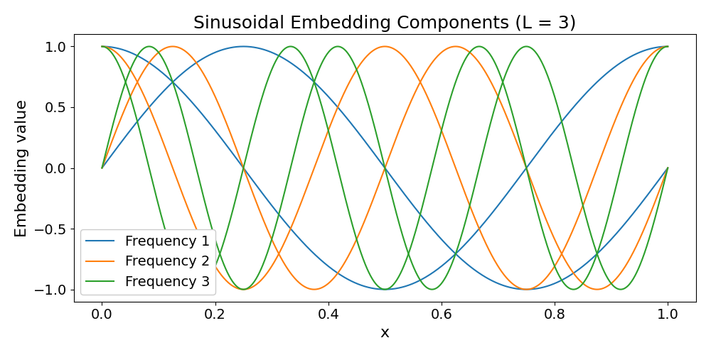
Below, we visualize the sinusoidal embeddings for a spatial input domain \(\vec{x} \in[0,1]\) consisting of 1000 equally spaced points, using \(L = 3\) frequency levels.
# Import required libraries
import torch
import matplotlib.pyplot as plt
import numpy as np
from neuralop.layers.embeddings import SinusoidalEmbedding

# Set default font sizes for better readability
plt.rcParams.update(
    {
        "font.size": 14,
        "axes.titlesize": 18,
        "axes.labelsize": 16,
        "xtick.labelsize": 14,
        "ytick.labelsize": 14,
        "legend.fontsize": 14,
    }
)

device = "cpu"

# Define a spatial domain and number of frequencies
# Create 1000 equally spaced points in [0, 1]
#  and normalize to [0, 2π] for proper sinusoidal embedding
x = torch.linspace(0, 1, 1000)
x_normalized = torch.linspace(0, 2 * torch.pi, len(x))
# Number of frequency levels for the embedding
L = 3

# Check if the number of frequencies satisfies the Nyquist-Criterion
if L < len(x_normalized) / 2:
    print(f"Nyquist-Shannon sampling theorem is satisfied for the given number of frequencies {L}.")
else:
    print(f"Nyquist-Shannon sampling theorem is violated for the given number of frequencies {L}.")

# Build embedding: [sin(x), cos(x), sin(2x), cos(2x), ...]
# Each frequency level contributes a sine and cosine pair
g = []
for l in range(1, L + 1):
    g.append(torch.sin(l * x_normalized))
    g.append(torch.cos(l * x_normalized))

# Construct input by concatenating the original input and the embedding
# This preserves the original coordinates while adding spectral information
input_arr = np.asarray([x, *g])
input_tensor = torch.tensor(input_arr)

# Plot the embedding components
colors = plt.cm.tab10.colors

plt.figure(figsize=(10, 5))
for freq_idx in range(L):
    color = colors[freq_idx % len(colors)]
    sin_idx = 2 * freq_idx + 1
    cos_idx = 2 * freq_idx + 2

    plt.plot(x, input_tensor[sin_idx], color=color, label=f"Frequency {freq_idx + 1}")
    plt.plot(x, input_tensor[cos_idx], color=color)

plt.xlabel("x", fontsize=16)
plt.ylabel("Embedding value", fontsize=16)
plt.title("Sinusoidal Embedding Components (L = 3)", fontsize=18)
plt.legend(loc="lower left", framealpha=1.0, fontsize=14)
plt.locator_params(axis="y", nbins=5)
plt.tight_layout()
plt.show()
Nyquist-Shannon sampling theorem is satisfied for the given number of frequencies 3.
Encoding Constant Parameters
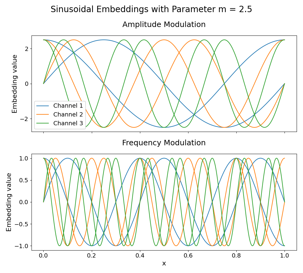
A particularly useful extension of sinusoidal embeddings is their ability to encode constant parameters. Consider a setting where you have a scalar parameter \(m\) (such as a material property, boundary condition, or physical constant) that you wish to feed into a model. Instead of treating \(m\) as a fixed scalar input, we can represent it using periodic functions, either by modulating the amplitude or the frequency of the sinusoidal components.
1. Amplitude Modulation: To encode \(m\) by scaling the amplitudes of the sinusoidal functions, we define the embedding as
where each element of the embedding \(g(\vec{x})\) is multiplied by \(m\).
2. Frequency Modulation: Alternatively, to encode \(m\) by scaling the frequencies, we define
where \(m\) multiplies the input argument of each sinusoidal component.
When encoding constant parameters through frequency modulation, care must be taken to ensure that the Nyquist criterion is satisfied. In this case, where the modulation factor \(m\) scales the frequencies, the Nyquist constraint becomes \(L < \frac{N}{2m}\).
Below, we demonstrate an example of encoding the parameter \(m = 2.5\) through both amplitude and frequency modulation.
# Define a spatial domain and number of frequencies
x = torch.linspace(0, 1, 1000)
x_normalized = torch.linspace(0, 2 * torch.pi, len(x))
L = 3

# Define parameter to encode
m = 2.5
m_tensor = torch.tensor([m])

# Check if the number of frequencies and parameter satisfies the Nyquist-Criterion
if L <= len(x_normalized) / (2 * m):
    print(f"Nyquist-Shannon sampling theorem is satisfied for the given parameter {m} and number of frequencies {L}.")
else:
    print(f"Nyquist-Shannon sampling theorem is violated for the given parameter {m} and number of frequencies {L}.")

# Build amplitude-modulated embedding: m * g(x)
g_amplitude = []
for l in range(1, L + 1):
    g_amplitude.append(torch.sin(l * x_normalized) * m_tensor)
    g_amplitude.append(torch.cos(l * x_normalized) * m_tensor)

# Build frequency-modulated embedding: g(m * x)
g_frequency = []
for l in range(1, L + 1):
    g_frequency.append(torch.sin(l * x_normalized * m_tensor))
    g_frequency.append(torch.cos(l * x_normalized * m_tensor))

# Convert to arrays for visualization
input_amplitude = torch.tensor(np.asarray([x, *g_amplitude]))
input_frequency = torch.tensor(np.asarray([x, *g_frequency]))

# Plot both embeddings
colors = plt.cm.tab10.colors
fig, axes = plt.subplots(2, 1, figsize=(10, 9), sharex=True)

## Amplitude modulation
for freq_idx in range(L):
    color = colors[freq_idx % len(colors)]
    sin_idx, cos_idx = 2 * freq_idx + 1, 2 * freq_idx + 2
    axes[0].plot(
        x, input_amplitude[sin_idx], color=color, label=f"Channel {freq_idx + 1}"
    )
    axes[0].plot(x, input_amplitude[cos_idx], color=color)
axes[0].set_title("Amplitude Modulation", fontsize=18, pad=20)
axes[0].set_ylabel("Embedding value", fontsize=16)
axes[0].legend(loc="lower left", framealpha=1.0, fontsize=14)
axes[0].locator_params(axis="y", nbins=5)

## Frequency modulation
for freq_idx in range(L):
    color = colors[freq_idx % len(colors)]
    sin_idx, cos_idx = 2 * freq_idx + 1, 2 * freq_idx + 2
    axes[1].plot(x, input_frequency[sin_idx], color=color, label=f"Channel {freq_idx + 1}")
    axes[1].plot(x, input_frequency[cos_idx], color=color)
axes[1].set_title("Frequency Modulation", fontsize=18, pad=20)
axes[1].set_ylabel("Embedding value", fontsize=16)
axes[1].set_xlabel("x", fontsize=16)
axes[1].locator_params(axis="y", nbins=5)

plt.suptitle(f"Sinusoidal Embeddings with Parameter m = {m}", y=0.98, fontsize=20)
plt.tight_layout()
plt.show()
Nyquist-Shannon sampling theorem is satisfied for the given parameter 2.5 and number of frequencies 3.
Neural Operator SinusoidalEmbedding Class
The neuralop library provides a unified sinusoidal positional embedding class,
neuralop.layers.embeddings.SinusoidalEmbedding, with the following embedding techniques:
transformer- Vaswani, A. et al (2017), “Attention Is All You Need”.nerf- Mildenhall, B. et al (2020), “NeRF: Representing Scenes as Neural Radiance Fields for View Synthesis”.
The SinusoidalEmbedding class expects inputs to be of shape
(batch_size, N, input_channels)or(N, input_channels)
Embedding Variants
Let \(\vec{x} \in \mathbb{R}^N\) denote a 1D input domain consisting of \(N\) discretized points. The embedding function \(g: \mathbb{R}^N \rightarrow \mathbb{R}^{N \times 2L}\) maps each input value \(x_n\) to a \(2L\)-dimensional vector composed of sine and cosine terms evaluated at different frequencies. Each embedding type defines these frequencies differently, leading to distinct representations.
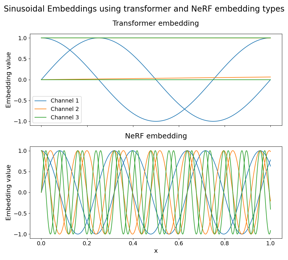
1. Transformer-style embedding: For \(0 \leq k < L\):
Here, \(\text{max_positions}\) controls the maximum position for the embedding.
2. NeRF-style embedding: For \(0 \leq k < L\):
In order to ensure that the Nyquist-Criterion is satisfied, for the Transformer-style embedding, the embedding frequencies should satisfy: \(f_{\max} < f_{\text{Nyquist}}\).
For the NeRF-style embedding:
Below, we include examples of using the SinusoidalEmbedding class with both the transformer- and NeRF-style embeddings.
# Define a spatial domain and the number of frequencies
x = torch.linspace(0, 1, 1000)
x_normalized = torch.linspace(0, 2 * torch.pi, len(x)).reshape(-1, 1)
L = 3

# Check if the number of frequencies satisfies the Nyquist-Criterion
if L <= 1 + torch.log2(torch.tensor(len(x_normalized) / 2)):
    print(f"Nyquist-Shannon sampling theorem is satisfied for the given number of frequencies {L}.")
else:
    print(f"Nyquist-Shannon sampling theorem is violated for the given number of frequencies {L}.")

# Define the transformer embedding
# max_positions controls the frequency scaling in transformer-style embeddings
max_positions = 1000
transformer_embedder = SinusoidalEmbedding(
    in_channels=1,
    num_frequencies=L,
    embedding_type="transformer",
    max_positions=max_positions,
).to(device)

# Apply transformer-style embedding
transformer_embedding = transformer_embedder(x_normalized).permute(1, 0)

# Define the NeRF embedding
nerf_embedder = SinusoidalEmbedding(
    in_channels=1, num_frequencies=L, embedding_type="nerf"
).to(device)

# Apply NeRF-style embedding, with the domain [0, 1]
nerf_embedding = nerf_embedder(x.reshape(-1, 1)).permute(1, 0)

# Plot both embeddings
colors = plt.cm.tab10.colors
fig, axes = plt.subplots(2, 1, figsize=(10, 9), sharex=True)

## Transformer embedding
for freq_idx in range(L):
    color = colors[freq_idx % len(colors)]
    sin_idx, cos_idx = 2 * freq_idx, 2 * freq_idx + 1

    axes[0].plot(x, transformer_embedding[sin_idx], color=color, label=f"Channel {freq_idx + 1}")
    axes[0].plot(x, transformer_embedding[cos_idx], color=color)

axes[0].set_title("Transformer embedding", fontsize=18, pad=20)
axes[0].set_ylabel("Embedding value", fontsize=16)
axes[0].legend(loc="lower left", framealpha=1.0, fontsize=14)
axes[0].locator_params(axis="y", nbins=5)

## NeRF embedding
for freq_idx in range(L):
    color = colors[freq_idx % len(colors)]
    sin_idx, cos_idx = 2 * freq_idx, 2 * freq_idx + 1

    axes[1].plot(x, nerf_embedding[sin_idx], color=color, label=f"Channel {freq_idx + 1}")
    axes[1].plot(x, nerf_embedding[cos_idx], color=color)

axes[1].set_title("NeRF embedding", fontsize=18, pad=20)
axes[1].set_xlabel("x", fontsize=16)
axes[1].set_ylabel("Embedding value", fontsize=16)
axes[1].locator_params(axis="y", nbins=5)

plt.suptitle("Sinusoidal Embeddings using transformer and NeRF embedding types", y=0.98, fontsize=20)
plt.tight_layout()
plt.show()
Nyquist-Shannon sampling theorem is satisfied for the given number of frequencies 3.
Encoding Constant Parameters with NeuralOp Class
Similar to the earlier illustrative examples, we can also encode a scalar parameter \(m\) before passing it to a model. Once again, care must be taken to ensure that the Nyquist criterion is satisfied.
In the Transformer-style embedding, to avoid aliasing, the embedding frequencies should still satisfy
For the NeRF-style embedding, the modified constraint becomes:
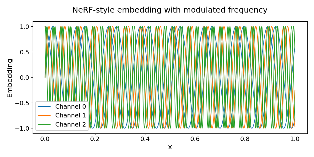
Below, we demonstrate an example of encoding the parameter \(m = 2.5\) through frequency modulation of the NeRF-style embedding.
# Define a spatial domain and the number of frequencies
x = torch.linspace(0, 1, 1000)
L = 3

# Define the parameter to encode
m = 2.5
m_tensor = torch.tensor([m])

# Check if the number of frequencies and parameter satisfies the Nyquist-Criterion
if L <= 1 + torch.log2(torch.tensor(len(x) / (2 * m))):
    print(f"Nyquist-Shannon sampling theorem is satisfied for the given parameter {m} and number of frequencies {L}.")
else:
    print(f"Nyquist-Shannon sampling theorem is violated for the given parameter {m} and number of frequencies {L}.")

# Define the NeRF embedding
nerf_embedder = SinusoidalEmbedding(
    in_channels=1, num_frequencies=L, embedding_type="nerf"
).to(device)

# Apply frequency modulation: multiply input, with the domain [0, 1], by parameter before embedding
# This scales all frequencies by the parameter m
nerf_embedding = nerf_embedder(x.reshape(-1, 1) * m_tensor).permute(1, 0)

# Plot the embedding
colors = plt.cm.tab10.colors

plt.figure(figsize=(10, 5))
for freq_idx in range(L):
    color = colors[freq_idx % len(colors)]
    sin_idx = 2 * freq_idx
    cos_idx = 2 * freq_idx + 1

    plt.plot(x, nerf_embedding[sin_idx], color=color, label=f"Channel {freq_idx}")
    plt.plot(x, nerf_embedding[cos_idx], color=color)

plt.xlabel("x", fontsize=16)
plt.ylabel("Embedding", fontsize=16)
plt.title("NeRF-style embedding with modulated frequency", fontsize=18, pad=20)
plt.legend(loc="lower left", framealpha=1.0, fontsize=14)
plt.locator_params(axis="y", nbins=5)
plt.tight_layout()
plt.show()
Nyquist-Shannon sampling theorem is satisfied for the given parameter 2.5 and number of frequencies 3.
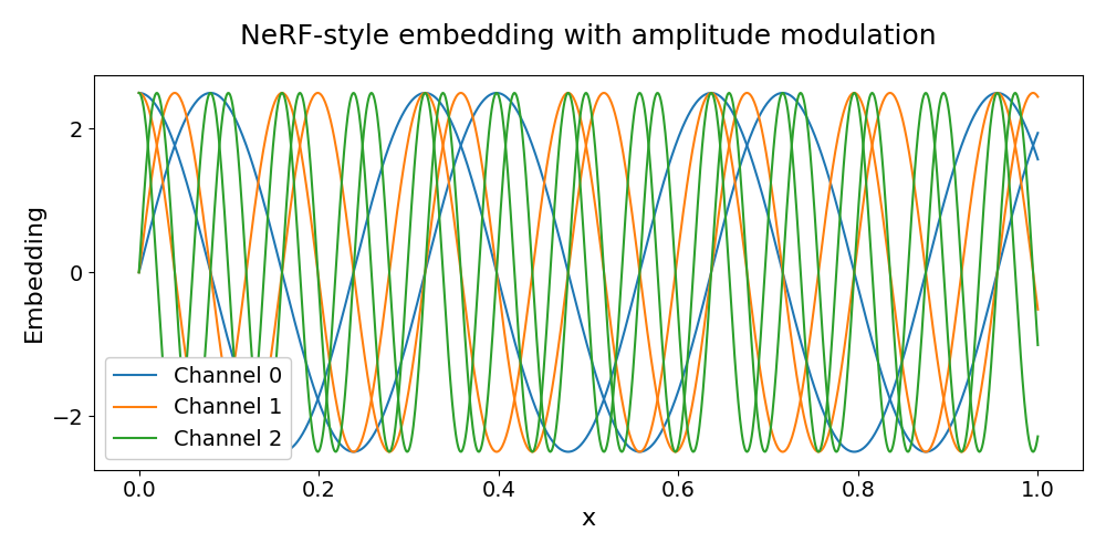
Similarly, we can encode the parameter \(m = 2.5\) through amplitude modulation, where we show an example using the NeRF-style embedding below.
# Define a spatial domain and the number of frequencies
x = torch.linspace(0, 1, 1000)
L = 3

# Define the parameter to encode
m = 2.5
m_tensor = torch.tensor([m])

# Check if the number of frequencies and parameter satisfies the Nyquist-Criterion
if L <= 1 + torch.log2(torch.tensor(len(x) / 2)):
    print(f"Nyquist-Shannon sampling theorem is satisfied for the given number of frequencies {L}.")
else:
    print(f"Nyquist-Shannon sampling theorem is violated for the given number of frequencies {L}.")

# Define the embedding
nerf_embedder = SinusoidalEmbedding(
    in_channels=1, num_frequencies=L, embedding_type="nerf"
).to(device)

# Apply amplitude modulation: multiply embedding, with the domain [0, 1], by parameter after computation
# This scales all embedding components by the parameter m
nerf_embedding = nerf_embedder(x.reshape(-1, 1)).permute(1, 0) * m_tensor

# Plot the embedding
colors = plt.cm.tab10.colors

plt.figure(figsize=(10, 5))
for freq_idx in range(L):
    color = colors[freq_idx % len(colors)]
    sin_idx = 2 * freq_idx
    cos_idx = 2 * freq_idx + 1

    plt.plot(x, nerf_embedding[sin_idx], color=color, label=f"Channel {freq_idx}")
    plt.plot(x, nerf_embedding[cos_idx], color=color)

plt.xlabel("x", fontsize=16)
plt.ylabel("Embedding", fontsize=16)
plt.title("NeRF-style embedding with amplitude modulation", fontsize=18, pad=20)
plt.legend(loc="lower left", framealpha=1.0, fontsize=14)
plt.locator_params(axis="y", nbins=5)
plt.tight_layout()
plt.show()
Nyquist-Shannon sampling theorem is satisfied for the given number of frequencies 3.
Application to Fourier Neural Operators (FNOs)
Fourier Neural Operators (FNOs) learn mappings between functions by operating in the frequency domain. They use the Fourier transform to express data as combinations of sine and cosine components, enabling them to capture complex, multi-scale interactions across frequencies. Given that sinusoidal embeddings also lift low-dimensional data into a richer spectral representation, they complement FNOs naturally. This synergy makes sinusoidal embeddings particularly effective for neural operator architectures.
In the general setting for neural operators, we strongly recommend choosing the number of frequencies \(L\) such that the Nyquist-Criterion is not violated. This can be done by following the guidelines we provided earlier for selecting \(L\) in both transformer-style and NeRF-style embeddings.
When dealing with FNOs with a specified number of Fourier modes, \(\text{n_modes}\), the highest embedded frequency should ideally also remain below \(\text{n_modes}\), as higher frequencies will be zeroed out and not acted upon by the spectral convolution operation.
For the NeRF-style embedding, this condition leads to an explicit upper bound on \(L\):
Setup in Higher Dimensions
Let \(X \in \mathbb{R}^{d \times N}\) denote a \(d\)-dimensional input domain consisting of \(N\) discretised points, where each row \(\vec{x}_{i} \in \mathbb{R}^N\) corresponds to the sampled coordinates along the \(i\)-th spatial or temporal dimension. Thus, each column of \(X\) represents a single point \(\vec{x}_{:,j} \in \mathbb{R}^d\) in the \(d\)-dimensional domain.
Building on the 1D embedding function \(g\) introduced earlier, we define the multi-dimensional embedding
where each \(\vec{x}_i\) denotes the sampled domain along the \(i\)-th input dimension.
The multi-dimensional embedding function \(h\) applies the 1D embedding function \(g\) independently to each coordinate dimension and concatenates the resulting embeddings along the feature axis. This approach allows the model to capture frequency patterns along each dimension separately while maintaining the overall structure.
Below, we include an example of using the SinusoidalEmbedding class to construct both transformer- and NeRF-style embeddings for a 3D input.
# Define a 1D spatial domain and construct 3D input by repeating the 1D domain
dim = 3
x_1d = torch.linspace(0, 1, 1000)
# For transformer: normalize to [0, 2π] and repeat for 3D input, shape (N, 3)
x_normalized_1d = torch.linspace(0, 2 * torch.pi, x_1d.size(0), device=x_1d.device).unsqueeze(1)
x_normalized = x_normalized_1d.repeat(1, dim)
# For NeRF: coordinates in [0, 1] per dimension, shape (N, 3)
x_3d = x_1d.unsqueeze(1).repeat(1, dim)

# Define the number of frequencies
L = 3

# Check if the number of frequencies satisfies the Nyquist-Criterion
# For multi-dimensional inputs, the constraint applies to each dimension independently
if L <= 1 + torch.log2(torch.tensor(len(x_3d) / 2)):
    print(f"Nyquist-Shannon sampling theorem is satisfied for the given number of frequencies {L}.")
else:
    print(f"Nyquist-Shannon sampling theorem is violated for the given number of frequencies {L}.")

# Transformer-style 3D embedding: use normalized coordinates [0, 2π]
max_positions = 1000
transformer_embedder = SinusoidalEmbedding(
    in_channels=dim,
    num_frequencies=L,
    embedding_type="transformer",
    max_positions=max_positions,
).to(device)
transformer_embedding = transformer_embedder(x_normalized).permute(1, 0)

# NeRF-style 3D embedding: use coordinates in [0, 1] per dimension
nerf_embedder = SinusoidalEmbedding(
    in_channels=dim, num_frequencies=L, embedding_type="nerf"
).to(device)
nerf_embedding = nerf_embedder(x_3d).permute(1, 0)
Nyquist-Shannon sampling theorem is satisfied for the given number of frequencies 3.
Total running time of the script: (0 minutes 0.834 seconds)