Note
Go to the end to download the full example code.
Fourier Differentiation
This tutorial demonstrates Fourier-based differentiation methods for computing derivatives of periodic functions. Fourier differentiation is crucial for:
Computing derivatives of functions with spectral accuracy
Implementing physics-informed loss functions
The FourierDiff class provides efficient implementations of spectral differentiation for periodic functions in 1D, 2D, and 3D domains.
Import the library
We first import our neuralop library and required dependencies.
import torch
import numpy as np
import matplotlib.pyplot as plt
from neuralop.losses.differentiation import FourierDiff

device = torch.device("cuda" if torch.cuda.is_available() else "cpu")
Creating an example of periodic 1D curve
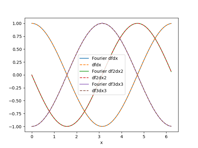
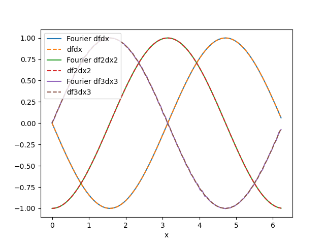
Here we consider sin(x) and cos(x), which are periodic on the interval [0, 2π]
L = 2 * torch.pi
x = torch.linspace(0, L, 101)[:-1]
f = torch.stack([torch.sin(x), torch.cos(x)], dim=0)
x_np = x.cpu().numpy()
Differentiate the signal
We use the FourierDiff class to differentiate the signal
fd1d = FourierDiff(dim=1, L=L, use_fc=False)
derivatives = fd1d.compute_multiple_derivatives(f, [1, 2, 3])
dfdx, df2dx2, df3dx3 = derivatives
Plot the results for sin(x)
plt.figure()
plt.plot(x_np, dfdx[0].squeeze().cpu().numpy(), label="Fourier dfdx")
plt.plot(x_np, np.cos(x_np), "--", label="dfdx")
plt.plot(x_np, df2dx2[0].squeeze().cpu().numpy(), label="Fourier df2dx2")
plt.plot(x_np, -np.sin(x_np), "--", label="df2dx2")
plt.plot(x_np, df3dx3[0].squeeze().cpu().numpy(), label="Fourier df3dx3")
plt.plot(x_np, -np.cos(x_np), "--", label="df3dx3")
plt.xlabel("x")
plt.legend()
plt.show()
Plot the results for cos(x)
plt.figure()
plt.plot(x_np, dfdx[1].squeeze().cpu().numpy(), label="Fourier dfdx")
plt.plot(x_np, -np.sin(x_np), "--", label="dfdx")
plt.plot(x_np, df2dx2[1].squeeze().cpu().numpy(), label="Fourier df2dx2")
plt.plot(x_np, -np.cos(x_np), "--", label="df2dx2")
plt.plot(x_np, df3dx3[1].squeeze().cpu().numpy(), label="Fourier df3dx3")
plt.plot(x_np, np.sin(x_np), "--", label="df3dx3")
plt.xlabel("x")
plt.legend()
plt.show()
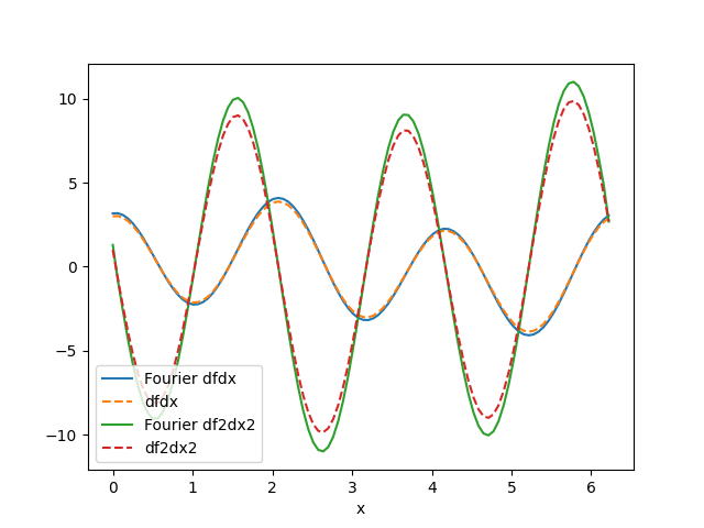
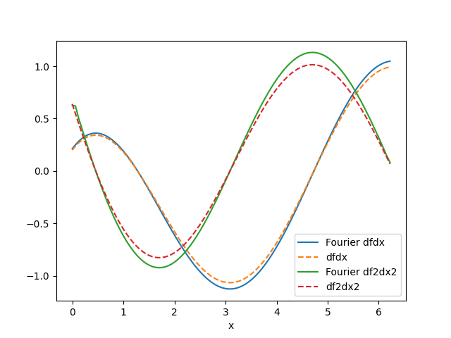
Creating an example of non-periodic 1D curve
Here we consider sin(3x)-cos(x) and exp(-0.8x)+sin(x)
L = 2 * torch.pi
x = torch.linspace(0, L, 101)[:-1]
f = torch.stack(
    [torch.sin(3 * x) - torch.cos(x), torch.exp(-0.8 * x) + torch.sin(x)], dim=0
)
x_np = x.cpu().numpy()
Differentiate the signal
We use the FourierDiff class with Fourier continuation to differentiate the signal
fd1d = FourierDiff(dim=1, L=L, use_fc="Legendre", fc_degree=4, fc_n_additional_pts=50)
derivatives = fd1d.compute_multiple_derivatives(f, [1, 2])
dfdx, df2dx2 = derivatives
Plot the results for sin(3x)-cos(x)
plt.figure()
plt.plot(x_np, dfdx[0].squeeze().cpu().numpy(), label="Fourier dfdx")
plt.plot(x_np, 3 * torch.cos(3 * x) + torch.sin(x), "--", label="dfdx")
plt.plot(x_np, df2dx2[0].squeeze().cpu().numpy(), label="Fourier df2dx2")
plt.plot(x_np, -9 * torch.sin(3 * x) + torch.cos(x), "--", label="df2dx2")
plt.xlabel("x")
plt.legend()
plt.show()
Plot the results for exp(-0.8x)+sin(x)
plt.figure()
plt.plot(x_np, dfdx[1].squeeze().cpu().numpy(), label="Fourier dfdx")
plt.plot(x_np, -0.8 * torch.exp(-0.8 * x) + torch.cos(x), "--", label="dfdx")
plt.plot(x_np, df2dx2[1].squeeze().cpu().numpy(), label="Fourier df2dx2")
plt.plot(x_np, 0.64 * torch.exp(-0.8 * x) - torch.sin(x), "--", label="df2dx2")
plt.xlabel("x")
plt.legend()
plt.show()
2D Fourier Differentiation Examples
Here we demonstrate the FourierDiff class for 2D functions
Creating an example of periodic 2D function
Here we consider f(x,y) = sin(x) * cos(y), which is periodic on the interval [0, 2π] × [0, 2π]
L_x, L_y = 2 * torch.pi, 2 * torch.pi
nx, ny = 180, 186
x = torch.linspace(0, L_x, nx, dtype=torch.float64)
y = torch.linspace(0, L_y, ny, dtype=torch.float64)
X, Y = torch.meshgrid(x, y, indexing="ij")

# Test function: f(x,y) = sin(x) * cos(y)
f_2d = torch.sin(X) * torch.cos(Y)
Differentiate the 2D signal
We use the FourierDiff class to compute derivatives
fd2d = FourierDiff(dim=2, L=(L_x, L_y))

# Compute derivatives
df_dx = fd2d.dx(f_2d)
df_dy = fd2d.dy(f_2d)
laplacian = fd2d.laplacian(f_2d)

# Expected analytical results for f(x,y) = sin(x) * cos(y)
df_dx_expected = torch.cos(X) * torch.cos(Y)
df_dy_expected = -torch.sin(X) * torch.sin(Y)
laplacian_expected = -2 * torch.sin(X) * torch.cos(Y)
Plot the 2D results
fig, axes = plt.subplots(2, 3, figsize=(15, 10))
fig.suptitle("2D Fourier Differentiation Results: f(x,y) = sin(x) * cos(y)")

# Compute consistent colorbar limits for each derivative pair
df_dx_min = min(df_dx.min().item(), df_dx_expected.min().item())
df_dx_max = max(df_dx.max().item(), df_dx_expected.max().item())
df_dy_min = min(df_dy.min().item(), df_dy_expected.min().item())
df_dy_max = max(df_dy.max().item(), df_dy_expected.max().item())

# Original function
im0 = axes[0, 0].imshow(f_2d.cpu().numpy())
axes[0, 0].set_title("Original: sin(x) * cos(y)")
plt.colorbar(im0, ax=axes[0, 0], shrink=0.57)

# ∂f/∂x computed
im1 = axes[0, 1].imshow(df_dx.cpu().numpy(), vmin=df_dx_min, vmax=df_dx_max)
axes[0, 1].set_title("∂f/∂x (computed)")
plt.colorbar(im1, ax=axes[0, 1], shrink=0.57)

# ∂f/∂x expected
im2 = axes[0, 2].imshow(df_dx_expected.cpu().numpy(), vmin=df_dx_min, vmax=df_dx_max)
axes[0, 2].set_title("∂f/∂x (expected: cos(x) * cos(y))")
plt.colorbar(im2, ax=axes[0, 2], shrink=0.57)

# ∂f/∂y computed
im3 = axes[1, 0].imshow(df_dy.cpu().numpy(), vmin=df_dy_min, vmax=df_dy_max)
axes[1, 0].set_title("∂f/∂y (computed)")
plt.colorbar(im3, ax=axes[1, 0], shrink=0.57)

# ∂f/∂y expected
im4 = axes[1, 1].imshow(df_dy_expected.cpu().numpy(), vmin=df_dy_min, vmax=df_dy_max)
axes[1, 1].set_title("∂f/∂y (expected: -sin(x) * sin(y))")
plt.colorbar(im4, ax=axes[1, 1], shrink=0.57)

# Laplacian
im5 = axes[1, 2].imshow(laplacian.cpu().numpy())
axes[1, 2].set_title("∇²f (computed)")
plt.colorbar(im5, ax=axes[1, 2], shrink=0.57)

plt.tight_layout()
plt.show()

3D Fourier Differentiation Examples
Here we demonstrate the FourierDiff class for 3D functions
Creating an example of periodic 3D function
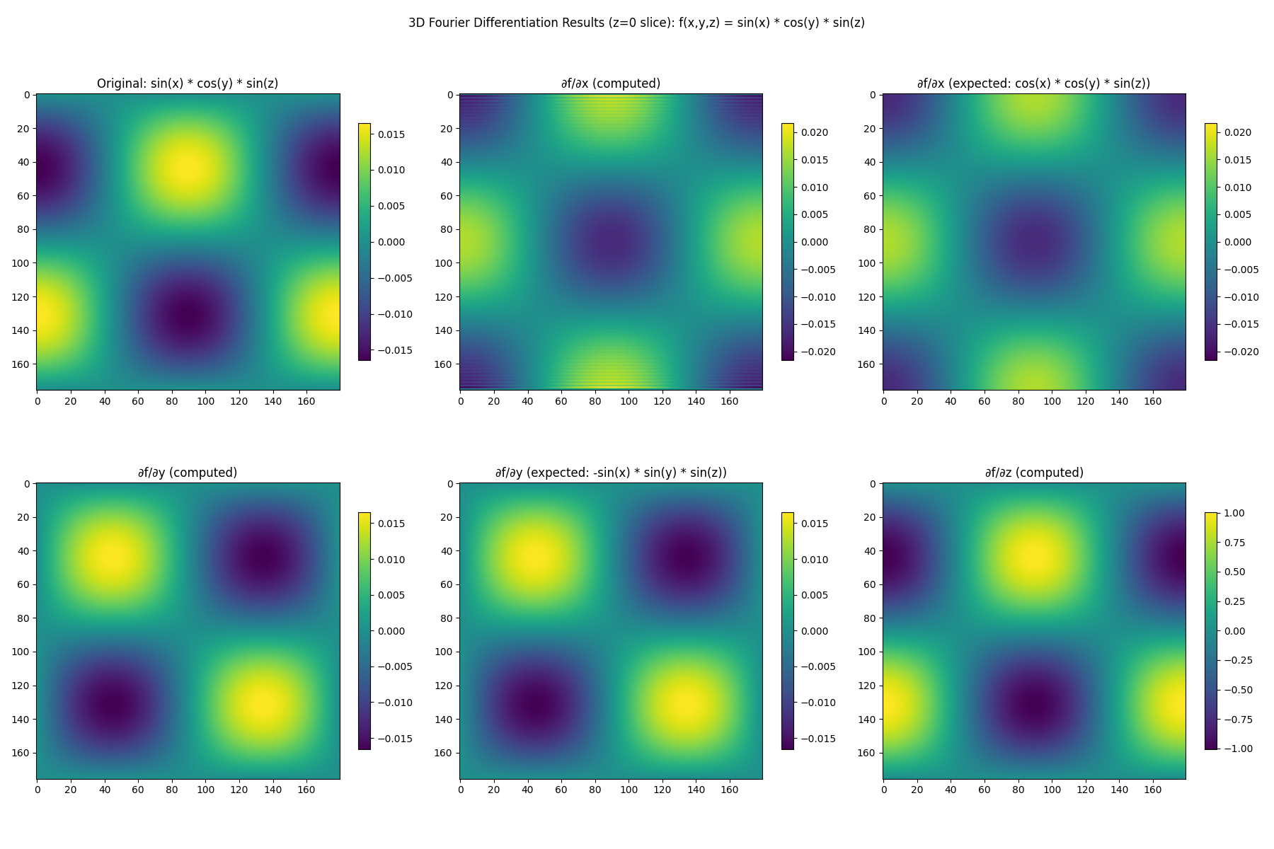
Here we consider f(x,y,z) = sin(x) * cos(y) * sin(z), which is periodic on [0, 2π]³
L_x, L_y, L_z = 2 * torch.pi, 2 * torch.pi, 2 * torch.pi
nx, ny, nz = 176, 180, 192
x = torch.linspace(0, L_x, nx, dtype=torch.float64)
y = torch.linspace(0, L_y, ny, dtype=torch.float64)
z = torch.linspace(0, L_z, nz, dtype=torch.float64)
X, Y, Z = torch.meshgrid(x, y, z, indexing="ij")

# Test function: f(x,y,z) = sin(x) * cos(y) * sin(z)
f_3d = torch.sin(X) * torch.cos(Y) * torch.sin(Z)

# Alternative: create tensor directly like in the test
f_3d_alt = torch.randn(nx, ny, nz, dtype=torch.float64)
Differentiate the 3D signal
We use the FourierDiff class to compute derivatives
fd3d = FourierDiff(dim=3, L=(L_x, L_y, L_z))

# Compute derivatives
df_dx_3d = fd3d.dx(f_3d)
df_dy_3d = fd3d.dy(f_3d)
df_dz_3d = fd3d.dz(f_3d)
laplacian_3d = fd3d.laplacian(f_3d)

# Expected analytical results for f(x,y,z) = sin(x) * cos(y) * sin(z)
df_dx_expected_3d = torch.cos(X) * torch.cos(Y) * torch.sin(Z)
df_dy_expected_3d = -torch.sin(X) * torch.sin(Y) * torch.sin(Z)
df_dz_expected_3d = torch.sin(X) * torch.cos(Y) * torch.cos(Z)
laplacian_expected_3d = -3 * torch.sin(X) * torch.cos(Y) * torch.sin(Z)
Plot a slice of the 3D results (z=0 plane)
z_slice_idx = nz // 2
fig, axes = plt.subplots(2, 3, figsize=(18, 12))
fig.suptitle("3D Fourier Differentiation Results (z=0 slice): f(x,y,z) = sin(x) * cos(y) * sin(z)")

# Compute consistent colorbar limits for each derivative pair at the z-slice
df_dx_3d_slice = df_dx_3d[:, :, z_slice_idx]
df_dx_expected_3d_slice = df_dx_expected_3d[:, :, z_slice_idx]
df_dy_3d_slice = df_dy_3d[:, :, z_slice_idx]
df_dy_expected_3d_slice = df_dy_expected_3d[:, :, z_slice_idx]

df_dx_3d_min = min(df_dx_3d_slice.min().item(), df_dx_expected_3d_slice.min().item())
df_dx_3d_max = max(df_dx_3d_slice.max().item(), df_dx_expected_3d_slice.max().item())
df_dy_3d_min = min(df_dy_3d_slice.min().item(), df_dy_expected_3d_slice.min().item())
df_dy_3d_max = max(df_dy_3d_slice.max().item(), df_dy_expected_3d_slice.max().item())

# Original function slice
im0 = axes[0, 0].imshow(f_3d[:, :, z_slice_idx].cpu().numpy())
axes[0, 0].set_title("Original: sin(x) * cos(y) * sin(z)")
plt.colorbar(im0, ax=axes[0, 0], shrink=0.57)

# ∂f/∂x slice
im1 = axes[0, 1].imshow(df_dx_3d_slice.cpu().numpy(), vmin=df_dx_3d_min, vmax=df_dx_3d_max)
axes[0, 1].set_title("∂f/∂x (computed)")
plt.colorbar(im1, ax=axes[0, 1], shrink=0.57)

# ∂f/∂x expected slice
im2 = axes[0, 2].imshow(df_dx_expected_3d_slice.cpu().numpy(), vmin=df_dx_3d_min, vmax=df_dx_3d_max)
axes[0, 2].set_title("∂f/∂x (expected: cos(x) * cos(y) * sin(z))")
plt.colorbar(im2, ax=axes[0, 2], shrink=0.57)

# ∂f/∂y slice
im3 = axes[1, 0].imshow(df_dy_3d_slice.cpu().numpy(), vmin=df_dy_3d_min, vmax=df_dy_3d_max)
axes[1, 0].set_title("∂f/∂y (computed)")
plt.colorbar(im3, ax=axes[1, 0], shrink=0.57)

# ∂f/∂y expected slice
im4 = axes[1, 1].imshow(df_dy_expected_3d_slice.cpu().numpy(), vmin=df_dy_3d_min, vmax=df_dy_3d_max)
axes[1, 1].set_title("∂f/∂y (expected: -sin(x) * sin(y) * sin(z))")
plt.colorbar(im4, ax=axes[1, 1], shrink=0.57)

# ∂f/∂z slice
im5 = axes[1, 2].imshow(df_dz_3d[:, :, z_slice_idx].cpu().numpy())
axes[1, 2].set_title("∂f/∂z (computed)")
plt.colorbar(im5, ax=axes[1, 2], shrink=0.57)

plt.tight_layout()
plt.show()
Total running time of the script: (0 minutes 4.229 seconds)