Note
Go to the end to download the full example code.
Normalization Layers
This tutorial demonstrates normalization layers designed for neural operators. Normalization is crucial for:
Stabilizing training dynamics
Accelerating convergence
Improving generalization
Handling different data distributions
The tutorial covers InstanceNorm, BatchNorm, and AdaIN layers, which are dimension-agnostic and flexible for various neural operator architectures.
Import dependencies
We import the necessary modules for working with normalization layers
import torch
import torch.nn as nn
import matplotlib.pyplot as plt
import numpy as np

from neuralop.layers.normalization_layers import InstanceNorm, BatchNorm, AdaIN

device = torch.device("cuda" if torch.cuda.is_available() else "cpu")
Understanding Normalization with 1D Functions
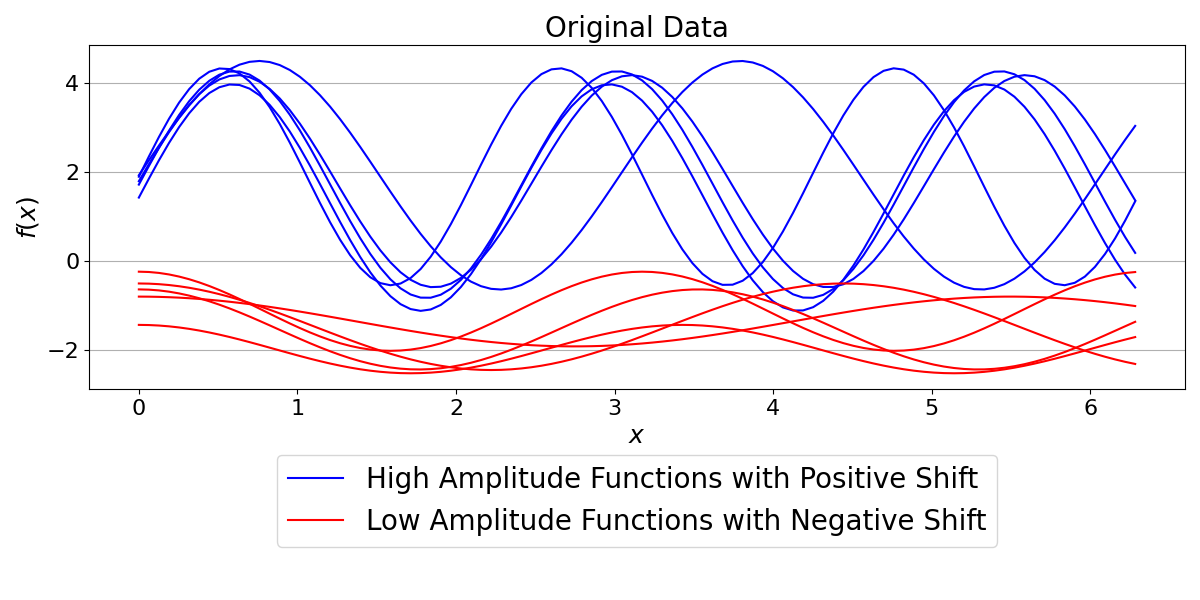
To clearly see how these layers work, we create a synthetic dataset of 1D functions. Our batch will consist of 10 functions. The first 5 will be sine waves with high amplitude and positive vertical shift, while the next 5 will be cosine waves with low amplitude and negative vertical shift.
n_samples = 10
n_points = 100
x = torch.linspace(0, 2 * torch.pi, n_points)
data = torch.zeros((n_samples, 1, n_points))

# Generate two groups of functions with different characteristics
for i in range(n_samples):
    if i < 5:
        # Group 1: High amplitude sine waves with positive vertical shift
        amplitude = np.random.uniform(2.0, 3.0)
        shift = np.random.uniform(1.0, 2.0)
        frequency = np.random.uniform(2.0, 3.0)
        data[i, 0, :] = amplitude * torch.sin(frequency * x) + shift
    else:
        # Group 2: Low amplitude cosine waves with negative vertical shift
        amplitude = np.random.uniform(0.5, 1.0)
        shift = np.random.uniform(-2.0, -1.0)
        frequency = np.random.uniform(1.0, 2.0)
        data[i, 0, :] = amplitude * torch.cos(frequency * x) + shift
Visualizing the original data
We plot the synthetic functions to see their different statistical properties. The blue functions have high amplitude and positive shift, while the red functions have low amplitude and negative shift.
plt.figure(figsize=(12, 6))
plt.title("Original Data", fontsize=20)
for i in range(n_samples):
    if i < 5:
        plt.plot(x, data[i, 0, :], "b-", label="High Amplitude Functions with Positive Shift" if i == 0 else "")
    else:
        plt.plot(x, data[i, 0, :], "r-", label="Low Amplitude Functions with Negative Shift" if i == 5 else "")

plt.legend(fontsize=20, loc="lower center", bbox_to_anchor=(0.5, -0.5), ncol=1)
plt.xlabel("$x$", fontsize=18)
plt.ylabel("$f(x)$", fontsize=18)
plt.xticks(fontsize=16)
plt.yticks(fontsize=16)
plt.locator_params(axis="y", nbins=5)
plt.grid(True, axis="y")
plt.subplots_adjust(bottom=0.2, top=0.9)
plt.tight_layout()
plt.show()
InstanceNorm
InstanceNorm normalizes each sample in the batch independently. This means it rescales each of the 10 functions to have a mean of 0 and a standard deviation of 1, regardless of the other functions in the batch. This is useful when the statistical properties of each sample are distinct and should be treated separately.
# Apply instance normalization
instance_norm = InstanceNorm()
data_in = instance_norm(data)

plt.figure(figsize=(12, 6))
plt.title("After InstanceNorm", fontsize=20)
for i in range(n_samples):
    y_plot = data_in[i, 0, :].detach().numpy()
    if i < 5:
        plt.plot(x, y_plot, "b-", label="High Amplitude Functions with Positive Shift" if i == 0 else "")
    else:
        plt.plot(x, y_plot, "r-", label="Low Amplitude Functions with Negative Shift" if i == 5 else "")
plt.legend(fontsize=20, loc="lower center", bbox_to_anchor=(0.5, -0.5), ncol=1)
plt.xlabel("$x$", fontsize=18)
plt.ylabel("$f(x)$", fontsize=18)
plt.xticks(fontsize=16)
plt.yticks(fontsize=16)
plt.locator_params(axis="y", nbins=5)
plt.grid(True, axis="y")
plt.subplots_adjust(bottom=0.2, top=0.9)
plt.tight_layout()
plt.show()
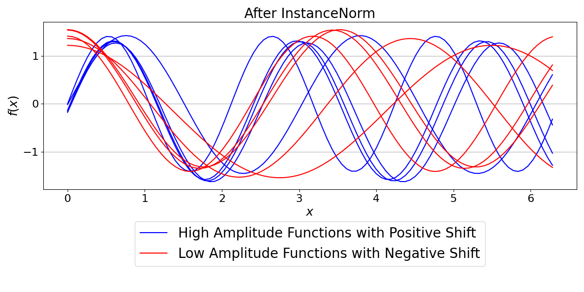
Notice how all functions are now perfectly scaled to the same range, centered around zero. The original differences in amplitude and shift between the functions have been completely removed by instance-wise normalization.
BatchNorm
BatchNorm normalizes the data across the entire batch. It computes a single mean and standard deviation for all 10 functions combined and uses these values to normalize all the data. This is the most common form of normalization and is effective when batch statistics are a good approximation of the overall data distribution.
# We need to specify the number of dimensions and features for BatchNorm
batch_norm = BatchNorm(n_dim=1, num_features=1)
data_bn = batch_norm(data)

plt.figure(figsize=(12, 6))
plt.title("After BatchNorm", fontsize=20)
for i in range(n_samples):
    y_plot = data_bn[i, 0, :].detach().numpy()
    if i < 5:
        plt.plot(x, y_plot, "b-", label="High Amplitude Functions with Positive Shift" if i == 0 else "")
    else:
        plt.plot(x, y_plot, "r-", label="Low Amplitude Functions with Negative Shift" if i == 5 else "")
plt.legend(fontsize=20, loc="lower center", bbox_to_anchor=(0.5, -0.5), ncol=1)
plt.xlabel("$x$", fontsize=18)
plt.ylabel("$f(x)$", fontsize=18)
plt.xticks(fontsize=16)
plt.yticks(fontsize=16)
plt.locator_params(axis="y", nbins=5)
plt.grid(True, axis="y")
plt.subplots_adjust(bottom=0.2, top=0.9)
plt.tight_layout()
plt.show()
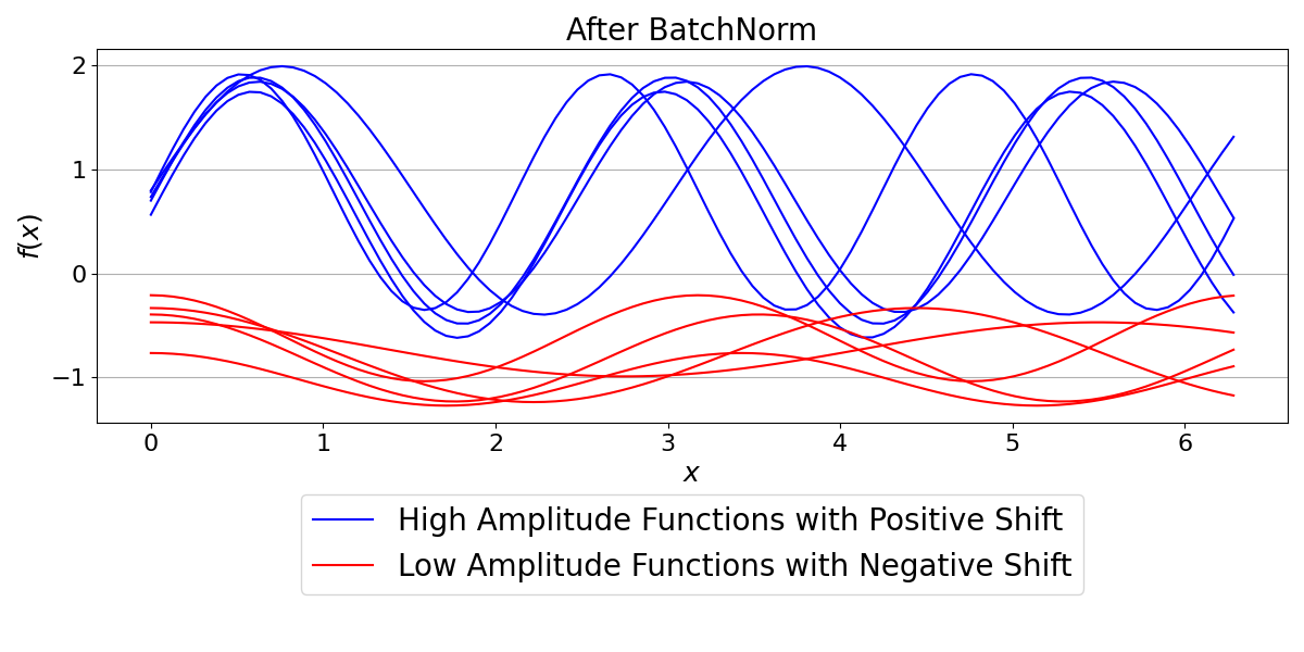
With BatchNorm, the relative differences between the two groups of functions are preserved. The high-amplitude functions are still visibly distinct from the low-amplitude ones, but the entire batch is now centered around a mean of zero with a standard deviation of one.
AdaIN (Adaptive Instance Normalization)
AdaIN is a more advanced normalization that allows for “style transfer.” It first normalizes an input (like InstanceNorm) and then applies a new style (a scaling weight and a shifting bias) derived from an external embedding vector. This is powerful for models where we want to control output characteristics based on a conditioning signal.
To guarantee a clear and deterministic result for this tutorial, we define our own simple MLP. This MLP maps our chosen style embeddings directly to a desired weight and bias.
content_function = torch.sin(2 * x).unsqueeze(0).unsqueeze(0)  # (1, 1, 100)


# A simple, predictable MLP that maps an embedding directly to a (weight, bias) pair
class ToyMLP(nn.Module):
    def forward(self, embedding):
        return embedding


# Style 1: A simple change in amplitude and mean (weight=2.0, bias=1.0)
style_embedding_1 = torch.tensor([2.0, 1.0])
# Style 2: A more complex change: inverting phase, shrinking, and shifting down (weight=-0.7, bias=-0.5)
style_embedding_2 = torch.tensor([-0.7, -0.5])

# The AdaIN layer needs to know the embedding dimension and number of input channels.
# We pass our toy MLP to have full control.
adain = AdaIN(embed_dim=2, in_channels=1, mlp=ToyMLP())

# Apply the first style
adain.set_embedding(style_embedding_1)
output_1 = adain(content_function)

# Apply the second style
adain.set_embedding(style_embedding_2)
output_2 = adain(content_function)

plt.figure(figsize=(12, 6))
plt.title("AdaIN for Style Transfer", fontsize=20)
plt.plot(x, content_function.squeeze().numpy(), "k--", label="Content Function")
plt.plot(x, output_1.squeeze().detach().numpy(), "g-", label="Style 1: Increased Amplitude, Positive Shift")
plt.plot(x, output_2.squeeze().detach().numpy(), "m-", label="Style 2: Inverted, Shrunk, Negative Shift")
plt.legend(fontsize=20, loc="lower center", bbox_to_anchor=(0.5, -0.7), ncol=1)
plt.xlabel("$x$", fontsize=18)
plt.ylabel("$f(x)$", fontsize=18)
plt.xticks(fontsize=16)
plt.yticks(fontsize=16)
plt.locator_params(axis="y", nbins=5)
plt.grid(True, axis="y")
plt.subplots_adjust(bottom=0.35, top=0.9)
plt.tight_layout()
plt.show()
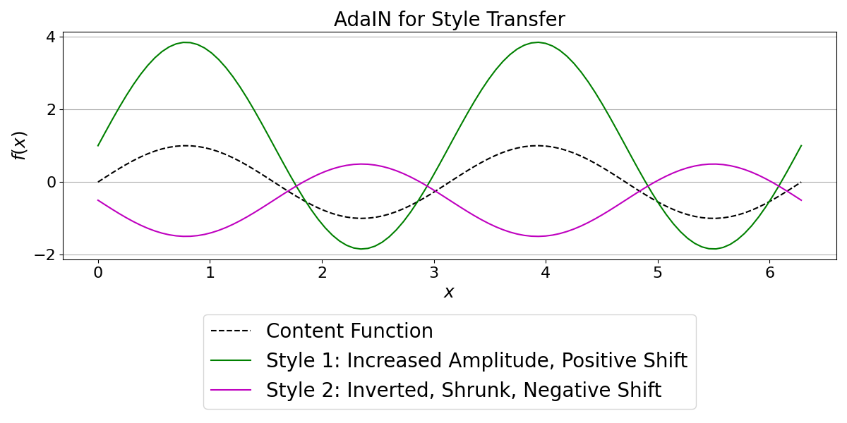
As you can see, the same content function is transformed into two very different outputs. Style 1 produces a simple sinusoidal wave with larger amplitude and positive shift. Style 2 produces a more complex transformation: the function is inverted (phase-shifted), its amplitude is reduced, and it’s shifted downwards. This demonstrates how AdaIN can modulate network layer output in diverse ways based on the style embedding.
Total running time of the script: (0 minutes 0.593 seconds)