Note
Go to the end to download the full example code.
Fourier Continuation
This tutorial demonstrates Fourier continuation methods for extending non-periodic functions to periodic ones, enabling efficient spectral analysis and neural operator applications. Fourier continuation is crucial for:
Converting non-periodic data to periodic form
Enabling spectral methods on arbitrary domains
Improving convergence of Fourier-based neural operators
Handling boundary conditions in spectral computations
The tutorial covers both FC-Legendre and FC-Gram methods for 1D, 2D, and 3D data.
Import the library
We first import our neuralop library and required dependencies.
import torch
import matplotlib.pyplot as plt
from matplotlib.lines import Line2D
from neuralop.layers.fourier_continuation import FCLegendre, FCGram


device = torch.device("cuda" if torch.cuda.is_available() else "cpu")
Creating an example of 1D non-periodic function
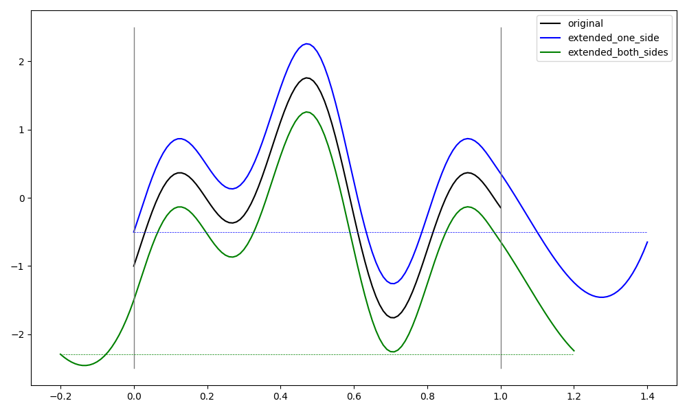
We consider f(x) = sin(16x) - cos(8x) on the interval [0,1]. This function is not periodic on [0,1], making it a good test case for Fourier continuation methods.
length_signal = 101  # Length of the original 1D signal
add_pts = 50  # Number of additional points for continuation
batch_size = 3  # Batch size for processing multiple signals

# Create the input signal
x = torch.linspace(0, 1, length_signal).repeat(batch_size, 1)
f = torch.sin(16 * x) - torch.cos(8 * x)
Extending the signal
We use the FC-Legendre and FC-Gram Fourier continuation layers to extend the signal.
# FC-Legendre: Uses Legendre polynomial basis for continuation
Extension_Legendre = FCLegendre(d=2, n_additional_pts=add_pts)
f_extend_Legendre = Extension_Legendre(f, dim=1)

# FC-Gram: Uses Gram polynomial basis for continuation
Extension_Gram = FCGram(d=4, n_additional_pts=add_pts)
f_extend_Gram = Extension_Gram(f, dim=1)
Visualizing the 1D Fourier continuation results
We plot the original function and both continuation methods to compare their effectiveness in creating smooth periodic extensions.
# Define the extended coordinates
x_extended = torch.linspace(-0.25, 1.25, 151)

# Adjust the extended functions for visualization purposes
f_extend_Legendre_adjusted = f_extend_Legendre - 0.6
f_extend_Gram_adjusted = f_extend_Gram + 0.6

plt.figure(figsize=(13, 6))
plt.plot(x[0], f[0], "k", label="Original Function", lw=2.2)
plt.plot(x_extended, f_extend_Gram_adjusted[0], "b", label="FC-Gram Extension", lw=2.2)
plt.plot(x_extended, f_extend_Legendre_adjusted[0], "g", label="FC-Legendre Extension", lw=2.2)
plt.plot([0, 0], [-2.9, 1.9], "-", color="gray", lw=1.5)
plt.plot([1, 1], [-2.9, 1.1], "-", color="gray", lw=1.5)
plt.plot([-0.25, 1.25], [f_extend_Legendre_adjusted[0, 0], f_extend_Legendre_adjusted[0, 0]], "--", color="g", lw=1.6)
plt.plot([-0.25, 1.25], [f_extend_Gram_adjusted[0, 0], f_extend_Gram_adjusted[0, 0]], "--", color="b", lw=1.6)
legend_elements = [
    Line2D([0], [0], color="k", lw=2.2, label="Original Function"),
    Line2D([0], [0], color="b", lw=2.2, label="FC-Gram Extension"),
    Line2D([0], [0], color="g", lw=2.2, label="FC-Legendre Extension"),
]
legend = plt.legend(handles=legend_elements, fontsize=19)
plt.xlim([-0.28, 1.31])
plt.ylim([-3.1, 2.6])
ax = plt.gca()
ax.spines["top"].set_visible(False)
ax.spines["right"].set_visible(False)
ax.tick_params(axis="x", which="major", labelsize=19)
ax.tick_params(axis="y", which="major", labelsize=19)
plt.xticks([-0.25, 0, 1, 1.25], ["-0.25", "0", "1", "1.25"])
plt.yticks([-2, 2])
plt.tight_layout()
plt.show()
Creating an example of 2D non-periodic function
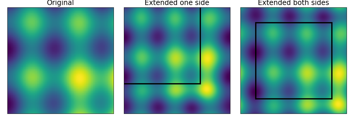
We consider f(x,y) = sin(12x) - cos(14y) + 3xy on the domain [0,1]×[0,1]. This function is not periodic on the unit square, making it suitable for testing 2D Fourier continuation methods.
length_signal = 101  # Length of the signal in each dimension
add_pts = 50  # Number of additional points for continuation in each dimension
batch_size = 3  # Batch size for processing multiple signals

# Create the 2D coordinate grids
x = torch.linspace(0, 1, length_signal).view(1, length_signal, 1).repeat(batch_size, 1, length_signal)
y = torch.linspace(0, 1, length_signal).view(1, 1, length_signal).repeat(batch_size, length_signal, 1)

# Define the 2D test function
f = torch.sin(12 * x) - torch.cos(14 * y) + 3 * x * y
Extending the signal
We use the FC-Legendre and FC-Gram Fourier continuation layers to extend the signal.
# FC-Legendre: Uses Legendre polynomial basis for 2D continuation
Extension_Legendre = FCLegendre(d=3, n_additional_pts=add_pts)
f_extend_Legendre = Extension_Legendre(f, dim=2)

# FC-Gram: Uses Gram polynomial basis for 2D continuation
Extension_Gram = FCGram(d=3, n_additional_pts=add_pts)
f_extend_Gram = Extension_Gram(f, dim=2)
Visualizing the 2D Fourier continuation results
We plot the original function and both continuation methods to compare their effectiveness in creating smooth 2D periodic extensions. Black lines delineate the original domain boundaries.
fig, axs = plt.subplots(figsize=(15, 5), nrows=1, ncols=3)

# Plot the original function
axs[0].imshow(f[0])
axs[0].set_title(r"Original Function", fontsize=15.5)
axs[1].imshow(f_extend_Legendre[0])
axs[1].plot([add_pts//2, length_signal + add_pts//2], [add_pts//2, add_pts//2], "-", color="k", lw=3)
axs[1].plot([add_pts//2, add_pts//2], [add_pts//2, length_signal + add_pts//2], "-", color="k", lw=3)
axs[1].plot([add_pts//2, length_signal + add_pts//2], [length_signal + add_pts//2, length_signal + add_pts//2], "-", color="k", lw=3)
axs[1].plot([length_signal + add_pts//2, length_signal + add_pts//2], [add_pts//2, length_signal + add_pts//2], "-", color="k", lw=3)
axs[1].set_title(r"FC-Legendre Extension", fontsize=15.5)
axs[2].imshow(f_extend_Gram[0])
axs[2].plot([add_pts//2, length_signal + add_pts//2], [add_pts//2, add_pts//2], "-", color="k", lw=3)
axs[2].plot([add_pts//2, add_pts//2], [add_pts//2, length_signal + add_pts//2], "-", color="k", lw=3)
axs[2].plot([add_pts//2, length_signal + add_pts//2], [length_signal + add_pts//2, length_signal + add_pts//2], "-", color="k", lw=3)
axs[2].plot([length_signal + add_pts//2, length_signal + add_pts//2], [add_pts//2, length_signal + add_pts//2], "-", color="k", lw=3)
axs[2].set_title(r"FC-Gram Extension", fontsize=15.5)
for ax in axs.flat:
    ax.set_xticks([])
    ax.set_yticks([])
plt.subplots_adjust(wspace=0.05)  # Reduce white space between plots
plt.show()
Creating an example of a 3D function
Here we consider f(x,y,z) = exp(-2z) + 2xz + sin(12xy) + y sin(10yz) which is not periodic on [0,1]x[0,1]x[0,1]
batch_size = 2
length_signal = 101
add_pts = 50

# Create 3D grid
x = torch.linspace(0, 1, length_signal).view(1, length_signal, 1, 1).repeat(batch_size, 1, length_signal, length_signal)
y = torch.linspace(0, 1, length_signal).view(1, 1, length_signal, 1).repeat(batch_size, length_signal, 1, length_signal)
z = torch.linspace(0, 1, length_signal).view(1, 1, 1, length_signal).repeat(batch_size, length_signal, length_signal, 1)

# Create 3D function
f = torch.exp(-2 * z) + 2 * z * x + torch.sin(12 * x * y) + y * torch.sin(10 * y * z)
Extending the signal
We use the FC-Legendre and FC-Gram Fourier continuation layers to extend the signal.
Extension_Legendre = FCLegendre(d=3, n_additional_pts=add_pts)
f_extend_Legendre = Extension_Legendre(f, dim=3)

Extension_Gram = FCGram(d=3, n_additional_pts=add_pts)
f_extend_Gram = Extension_Gram(f, dim=3)
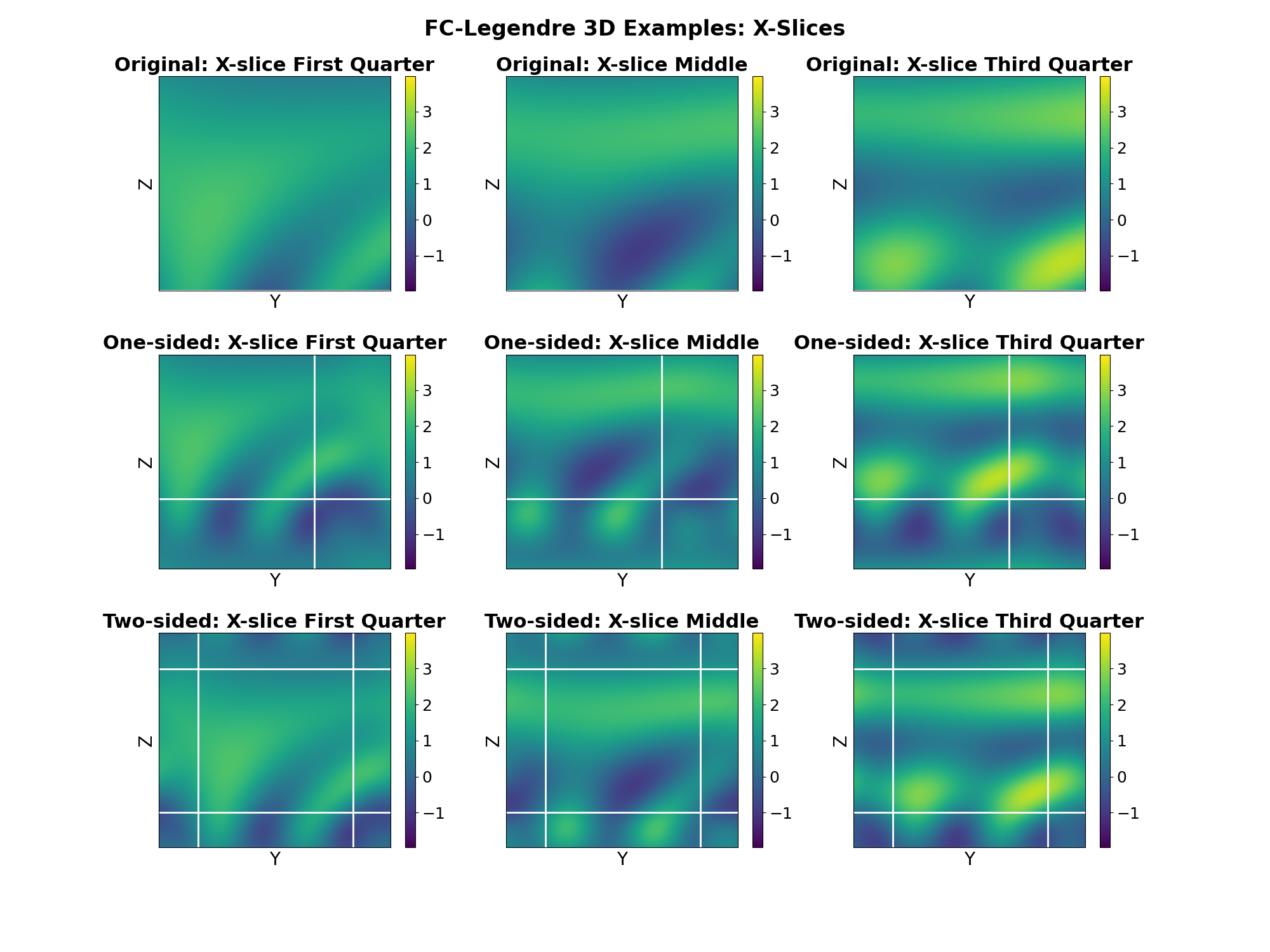
Plot the FC-Legendre and FC-Gram results for 3D
We also add white lines to deliminate the original signal
f_min = f.min().item()
f_max = f.max().item()
f_ext_legendre_min = f_extend_Legendre.min().item()
f_ext_legendre_max = f_extend_Legendre.max().item()
f_ext_gram_min = f_extend_Gram.min().item()
f_ext_gram_max = f_extend_Gram.max().item()
global_min = min(f_min, f_ext_legendre_min, f_ext_gram_min)
global_max = max(f_max, f_ext_legendre_max, f_ext_gram_max)
Figure for X slices
fig = plt.figure(figsize=(24, 20))
slice_indices = [length_signal//4, length_signal//2, 3*length_signal//4]
slice_names = ["First Quarter", "Middle", "Third Quarter"]

for i, (idx, name) in enumerate(zip(slice_indices, slice_names)):
    # Original function - X-slice
    ax = fig.add_subplot(3, 3, i + 1)
    im = ax.imshow(f[0, idx, :, :].numpy(), cmap="viridis", aspect="auto", vmin=global_min, vmax=global_max)
    ax.set_title(f"Original: X-slice {name}", fontsize=22, fontweight="bold")
    ax.set_xlabel("Y", fontsize=20)
    ax.set_ylabel("Z", fontsize=20)
    ax.set_xticks([])
    ax.set_yticks([])
    cbar = plt.colorbar(im, ax=ax)
    cbar.ax.tick_params(labelsize=18)

    # FC-Legendre extension - X-slice
    ax = fig.add_subplot(3, 3, i + 4)
    ext_idx = idx + add_pts//2
    im = ax.imshow(f_extend_Legendre[0, ext_idx, :, :].numpy(), cmap="viridis", aspect="auto", vmin=global_min, vmax=global_max)
    ax.set_title(f"FC-Legendre: X-slice {name}", fontsize=22, fontweight="bold")
    ax.set_xlabel("Y", fontsize=20)
    ax.set_ylabel("Z", fontsize=20)
    # Draw boundary lines
    ax.axhline(y=add_pts//2, color="white", linewidth=2, linestyle="-")
    ax.axhline(y=length_signal + add_pts//2, color="white", linewidth=2, linestyle="-")
    ax.axvline(x=add_pts//2, color="white", linewidth=2, linestyle="-")
    ax.axvline(x=length_signal + add_pts//2, color="white", linewidth=2, linestyle="-")
    ax.set_xticks([])
    ax.set_yticks([])
    cbar = plt.colorbar(im, ax=ax)
    cbar.ax.tick_params(labelsize=18)

    # FC-Gram extension - X-slice
    ax = fig.add_subplot(3, 3, i + 7)
    im = ax.imshow(f_extend_Gram[0, ext_idx, :, :].numpy(), cmap="viridis", aspect="auto", vmin=global_min, vmax=global_max)
    ax.set_title(f"FC-Gram: X-slice {name}", fontsize=22, fontweight="bold")
    ax.set_xlabel("Y", fontsize=20)
    ax.set_ylabel("Z", fontsize=20)
    # Draw boundary lines
    ax.axhline(y=add_pts//2, color="white", linewidth=2, linestyle="-")
    ax.axhline(y=length_signal + add_pts//2, color="white", linewidth=2, linestyle="-")
    ax.axvline(x=add_pts//2, color="white", linewidth=2, linestyle="-")
    ax.axvline(x=length_signal + add_pts//2, color="white", linewidth=2, linestyle="-")
    ax.set_xticks([])
    ax.set_yticks([])
    cbar = plt.colorbar(im, ax=ax)
    cbar.ax.tick_params(labelsize=18)

plt.subplots_adjust(hspace=0.15, wspace=0.05, top=0.95)
plt.show()
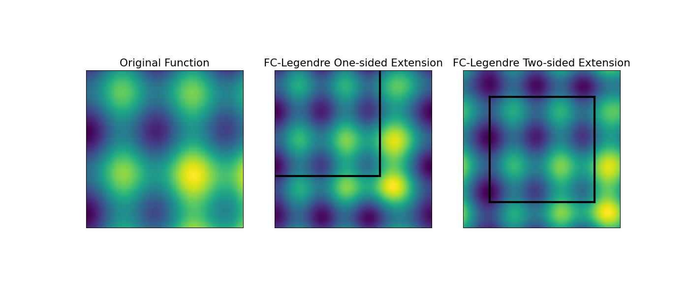
Figure for Y-slices
fig2 = plt.figure(figsize=(24, 20))

for i, (idx, name) in enumerate(zip(slice_indices, slice_names)):
    # Original function - Y-slice
    ax = fig2.add_subplot(3, 3, i + 1)
    im = ax.imshow(f[0, :, idx, :].numpy(), cmap="viridis", aspect="auto", vmin=global_min, vmax=global_max)
    ax.set_title(f"Original: Y-slice {name}", fontsize=22, fontweight="bold")
    ax.set_xlabel("X", fontsize=20)
    ax.set_ylabel("Z", fontsize=20)
    ax.set_xticks([])
    ax.set_yticks([])
    cbar = plt.colorbar(im, ax=ax)
    cbar.ax.tick_params(labelsize=18)

    # FC-Legendre extension - Y-slice
    ax = fig2.add_subplot(3, 3, i + 4)
    ext_idx = idx + add_pts//2
    im = ax.imshow(f_extend_Legendre[0, :, ext_idx, :].numpy(), cmap="viridis", aspect="auto", vmin=global_min, vmax=global_max)
    ax.set_title(f"FC-Legendre: Y-slice {name}", fontsize=22, fontweight="bold")
    ax.set_xlabel("X", fontsize=20)
    ax.set_ylabel("Z", fontsize=20)
    # Draw boundary lines
    ax.axhline(y=add_pts//2, color="white", linewidth=2, linestyle="-")
    ax.axhline(y=length_signal + add_pts//2, color="white", linewidth=2, linestyle="-")
    ax.axvline(x=add_pts//2, color="white", linewidth=2, linestyle="-")
    ax.axvline(x=length_signal + add_pts//2, color="white", linewidth=2, linestyle="-")
    ax.set_xticks([])
    ax.set_yticks([])
    cbar = plt.colorbar(im, ax=ax)
    cbar.ax.tick_params(labelsize=18)

    # FC-Gram extension - Y-slice
    ax = fig2.add_subplot(3, 3, i + 7)
    im = ax.imshow(f_extend_Gram[0, :, ext_idx, :].numpy(), cmap="viridis", aspect="auto", vmin=global_min, vmax=global_max)
    ax.set_title(f"FC-Gram: Y-slice {name}", fontsize=22, fontweight="bold")
    ax.set_xlabel("X", fontsize=20)
    ax.set_ylabel("Z", fontsize=20)
    # Draw boundary lines
    ax.axhline(y=add_pts//2, color="white", linewidth=2, linestyle="-")
    ax.axhline(y=length_signal + add_pts//2, color="white", linewidth=2, linestyle="-")
    ax.axvline(x=add_pts//2, color="white", linewidth=2, linestyle="-")
    ax.axvline(x=length_signal + add_pts//2, color="white", linewidth=2, linestyle="-")
    ax.set_xticks([])
    ax.set_yticks([])
    cbar = plt.colorbar(im, ax=ax)
    cbar.ax.tick_params(labelsize=18)

plt.subplots_adjust(hspace=0.15, wspace=0.05, top=0.95)
plt.show()
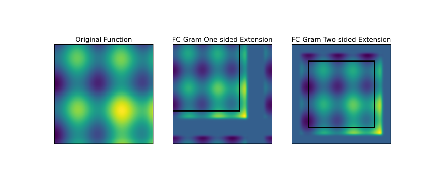
Figure for Z-slices
fig3 = plt.figure(figsize=(24, 20))

for i, (idx, name) in enumerate(zip(slice_indices, slice_names)):
    # Original function - Z-slice
    ax = fig3.add_subplot(3, 3, i + 1)
    im = ax.imshow(f[0, :, :, idx].numpy(), cmap="viridis", aspect="auto", vmin=global_min, vmax=global_max)
    ax.set_title(f"Original: Z-slice {name}", fontsize=22, fontweight="bold")
    ax.set_xlabel("X", fontsize=20)
    ax.set_ylabel("Y", fontsize=20)
    ax.set_xticks([])
    ax.set_yticks([])
    cbar = plt.colorbar(im, ax=ax)
    cbar.ax.tick_params(labelsize=18)

    # FC-Legendre extension - Z-slice
    ax = fig3.add_subplot(3, 3, i + 4)
    ext_idx = idx + add_pts//2
    im = ax.imshow(f_extend_Legendre[0, :, :, ext_idx].numpy(), cmap="viridis", aspect="auto", vmin=global_min, vmax=global_max)
    ax.set_title(f"FC-Legendre: Z-slice {name}", fontsize=22, fontweight="bold")
    ax.set_xlabel("X", fontsize=20)
    ax.set_ylabel("Y", fontsize=20)
    # Draw boundary lines
    ax.axhline(y=add_pts//2, color="white", linewidth=2, linestyle="-")
    ax.axhline(y=length_signal + add_pts//2, color="white", linewidth=2, linestyle="-")
    ax.axvline(x=add_pts//2, color="white", linewidth=2, linestyle="-")
    ax.axvline(x=length_signal + add_pts//2, color="white", linewidth=2, linestyle="-")
    ax.set_xticks([])
    ax.set_yticks([])
    cbar = plt.colorbar(im, ax=ax)
    cbar.ax.tick_params(labelsize=18)

    # FC-Gram extension - Z-slice
    ax = fig3.add_subplot(3, 3, i + 7)
    im = ax.imshow(f_extend_Gram[0, :, :, ext_idx].numpy(), cmap="viridis", aspect="auto", vmin=global_min, vmax=global_max)
    ax.set_title(f"FC-Gram: Z-slice {name}", fontsize=22, fontweight="bold")
    ax.set_xlabel("X", fontsize=20)
    ax.set_ylabel("Y", fontsize=20)
    # Draw boundary lines
    ax.axhline(y=add_pts//2, color="white", linewidth=2, linestyle="-")
    ax.axhline(y=length_signal + add_pts//2, color="white", linewidth=2, linestyle="-")
    ax.axvline(x=add_pts//2, color="white", linewidth=2, linestyle="-")
    ax.axvline(x=length_signal + add_pts//2, color="white", linewidth=2, linestyle="-")
    ax.set_xticks([])
    ax.set_yticks([])
    cbar = plt.colorbar(im, ax=ax)
    cbar.ax.tick_params(labelsize=18)

plt.subplots_adjust(hspace=0.15, wspace=0.05, top=0.95)
plt.show()
Total running time of the script: (0 minutes 2.378 seconds)