Visualizing computational fluid dynamics on a car

In this example we visualize a mesh drawn from the CarCFDDataset.

This tutorial demonstrates how to work with unstructured mesh data from computational fluid dynamics (CFD) simulations. We will explore the 3D geometry of a car and understand how pressure fields are distributed over the surface, which is crucial for aerodynamic analysis and neural operator applications.

The CarCFD dataset contains: - 3D triangular mesh data representing the car surface - Pressure fields computed from CFD simulations - Query points for neural operator training

Import dependencies

We first import our neuralop library and required dependencies.

import numpy as np
import torch
import matplotlib
import matplotlib.pyplot as plt
from neuralop.data.datasets import load_mini_car

font = {"size": 12}
matplotlib.rc("font", **font)

torch.manual_seed(0)
np.random.seed(0)

Understanding the data structure

The data in a MeshDataModule is structured as a dictionary of tensors and important scalar values encoding a 3D triangle mesh over the surface of a car. Each sample includes the coordinates of all triangle vertices and the centroids of each triangle face.

In this case, the creators used OpenFOAM to simulate the surface air pressure on car geometries in a wind tunnel. The 3D Navier-Stokes equations were simulated for a variety of inlet velocities over each surface using the OpenFOAM computational solver to predict pressure at every vertex on the mesh. Each sample here also has an inlet velocity scalar and a pressure field that maps 1-to-1 with the vertices on the mesh. The full CarCFDDataset is stored in triangle mesh files for downstream processing. For the sake of simplicity, we’ve packaged a few examples of the data after processing in tensor form to visualize here:

data_list = load_mini_car()
sample = data_list[0]
print(f"Available data keys: {sample.keys()}")

Available data keys: dict_keys(['vertices', 'vertex_normals', 'triangle_normals', 'centroids', 'triangle_areas', 'distance', 'closest_points', 'normalized_triangle_areas', 'press', 'query_points'])

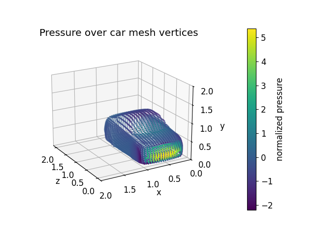
Visualizing the car surface with pressure distribution

Let’s take a look at the vertices and pressure values to understand the 3D structure and how pressure varies across the car surface.

fig = plt.figure(figsize=(10, 8))
ax = fig.add_subplot(projection="3d")

# By default the data is normalized into the unit cube. To get a
# better look at it, we scale the z-direction up.
scatter = ax.scatter(sample["vertices"][:, 0], sample["vertices"][:, 1],
                     sample["vertices"][:, 2] * 2, s=2, c=sample["press"].numpy(), cmap="viridis")
ax.set_xlim(0,2)
ax.set_ylim(0,2)
ax.set_xlabel("x")
ax.set_ylabel("y")
ax.set_zlabel("z")
ax.view_init(elev=20, azim=150, roll=0, vertical_axis="y")
ax.set_title("Pressure distribution over car mesh vertices")
fig.colorbar(scatter, pad=0.2, label="normalized pressure", ax=ax)
plt.draw()

Pressure distribution over car mesh vertices

Understanding query points for neural operator training

Each sample in the CarCFDDataset also includes a set of latent query points on which we learn a function to enable learning with an FNO in the middle of our geometry-informed models. Let’s visualize the queries on top of the car from before:

fig = plt.figure(figsize=(8,10))
ax = fig.add_subplot(projection="3d")
scatter = ax.scatter(sample["vertices"][:, 0], sample["vertices"][:, 1], sample["vertices"][:, 2] * 2, s=4, label="Car surface")
queries = sample["query_points"].view(-1, 3) # unroll our cube tensor into a point cloud
ax.scatter(queries[:, 0], queries[:, 1], queries[:, 2] * 2, s=1, alpha=0.5, label="Latent queries")

ax.set_xlim(0, 2)
ax.set_ylim(0, 2)
ax.set_xlabel("x")
ax.set_ylabel("y")
ax.set_zlabel("z")
ax.legend()
ax.view_init(elev=20, azim=150, roll=0, vertical_axis="y")
ax.set_title("Query points and car surface vertices")

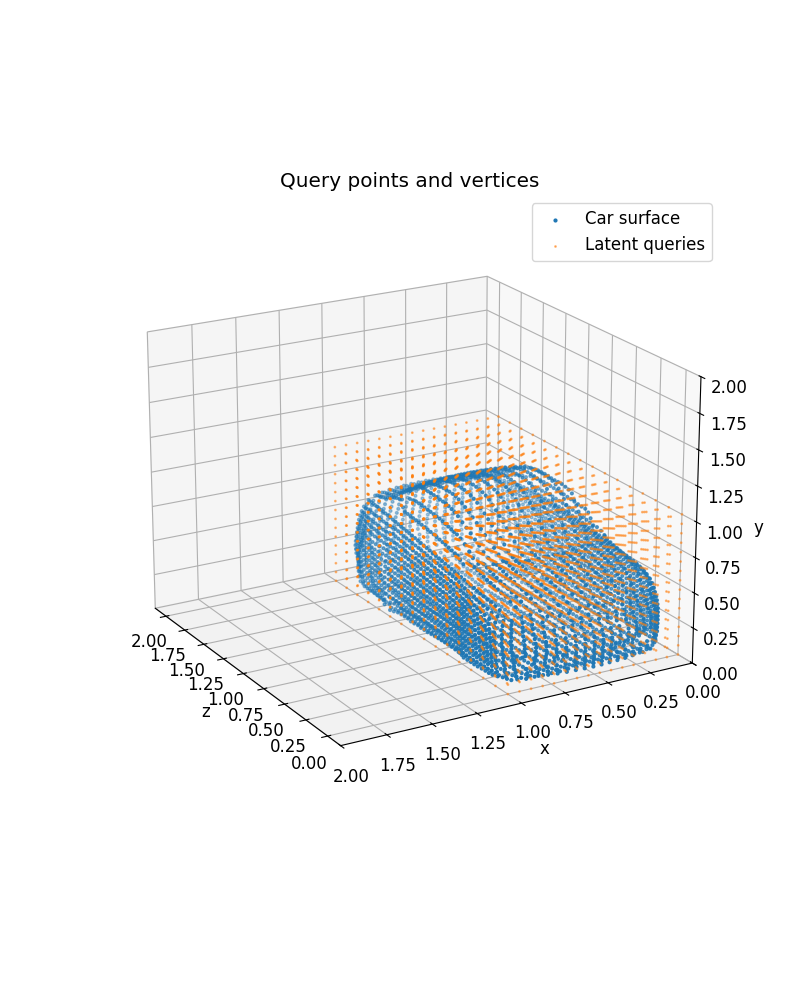
Text(0.5, 1.0, 'Query points and car surface vertices')

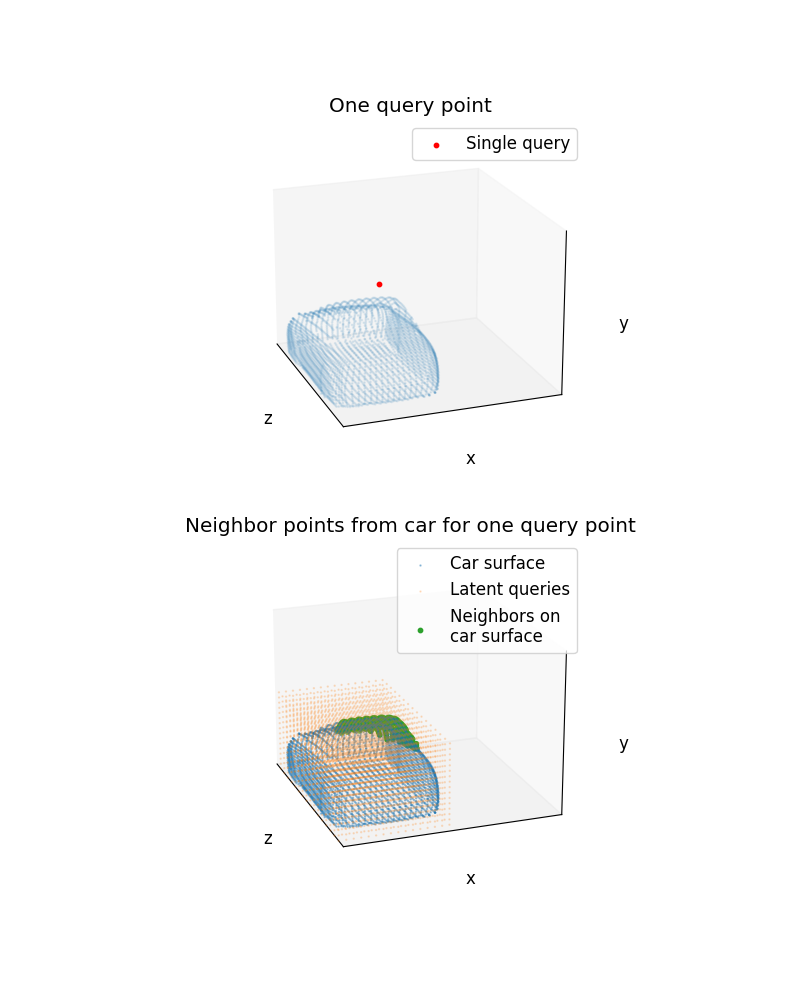
Neighbor search between 3D point clouds

In Neighbor Search for Graph Neural Operators we demonstrate our neighbor search on a simple 2D point cloud. Let’s try that again with our 3D car surface points here.

from neuralop.layers.neighbor_search import native_neighbor_search

verts = sample["vertices"]
query_point = queries[3300]
nbr_data = native_neighbor_search(data=verts, queries=query_point.unsqueeze(0), radius=0.5)

Let’s plot the new neighbors we just found on top of the car surface point cloud.

fig = plt.figure(figsize=(8, 10))
ax1 = fig.add_subplot(2, 1, 1, projection="3d")
ax2 = fig.add_subplot(2, 1, 2, projection="3d")
neighbors = verts[nbr_data["neighbors_index"]]

# Plotting just one query point vs. the car
ax1.scatter(verts[:, 0], verts[:, 1], verts[:, 2]*2, s=1, alpha=0.1)
ax1.scatter(query_point[0], query_point[1], query_point[2]*2, s=10, c="red", label="Single query")
ax1.view_init(elev=20, azim=-20, roll=0, vertical_axis="y")
ax1.legend()
ax1.set_xlim(0, 2)
ax1.set_ylim(0, 2)
ax1.set_xlabel("x")
ax1.set_ylabel("y")
ax1.set_zlabel("z")
ax1.view_init(elev=20, azim=-20, roll=0, vertical_axis="y")
ax1.grid(False)
ax1.set_title("One query point")

# Plotting all query points and neighbors
ax2.scatter(verts[:, 0], verts[:, 1], verts[:, 2]*2, s=0.5, alpha=0.4, label="Car surface")
ax2.scatter(queries[:, 0], queries[:, 1], queries[:, 2]*2, s=0.5, alpha=0.2, label="Latent queries")
ax2.scatter(neighbors[:, 0], neighbors[:, 1], neighbors[:, 2]*2, s=10, label="Neighbors on\ncar surface",)
ax2.legend()
ax2.set_xlim(0, 2)
ax2.set_ylim(0, 2)
ax2.set_xlabel("x")
ax2.set_ylabel("y")
ax2.set_zlabel("z")
ax2.view_init(elev=20, azim=-20, roll=0, vertical_axis="y")
ax2.set_title("Neighbor points from car for one query point")
ax2.grid(False)

for ax in ax1, ax2:
    ax.set_xticks([])
    ax.set_yticks([])
    ax.set_zticks([])
plt.draw()

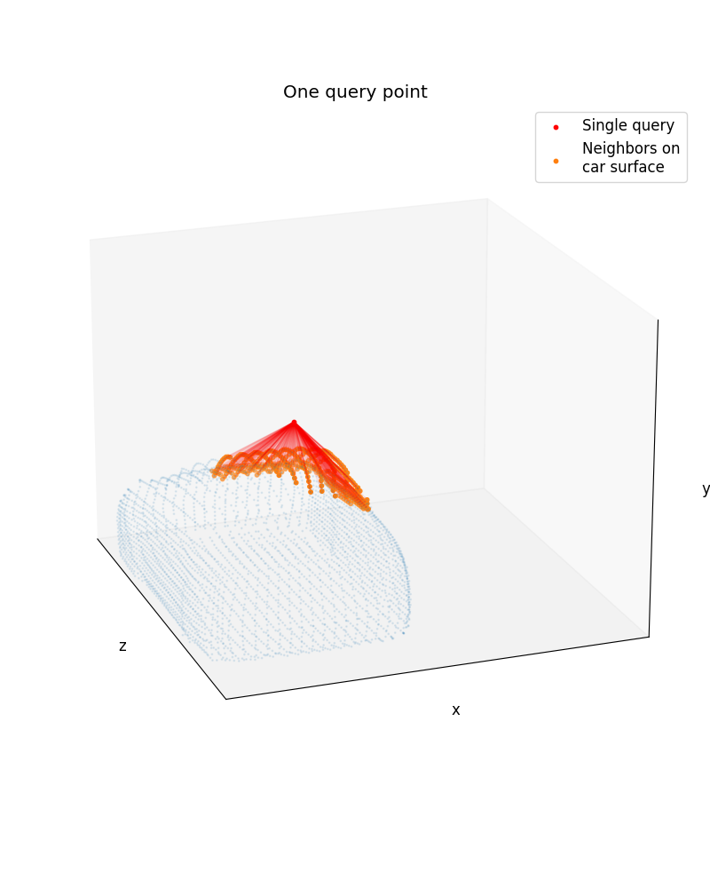
One query point, Neighbor points from car for one query point

Connecting neighbors to query

First, let’s make a simple utiltiy to add arrows to our 3D plot:

import numpy as np
from matplotlib import pyplot as plt
from matplotlib.patches import FancyArrowPatch
from mpl_toolkits.mplot3d import proj3d


class Arrow3D(FancyArrowPatch):
    def __init__(self, xs, ys, zs, *args, **kwargs):
        super().__init__((0, 0), (0, 0), *args, **kwargs)
        self._verts3d = xs, ys, zs

    def do_3d_projection(self, renderer=None):
        xs3d, ys3d, zs3d = self._verts3d
        xs, ys, zs = proj3d.proj_transform(xs3d, ys3d, zs3d, self.axes.M)
        self.set_positions((xs[0], ys[0]), (xs[1], ys[1]))

        return np.min(zs)


# Creating plots
fig = plt.figure(figsize=(8, 10))
ax1 = fig.add_subplot(projection="3d")
neighbors = verts[nbr_data["neighbors_index"]]

# Plotting just one query point vs. the car
ax1.scatter(verts[:, 0], verts[:, 1], verts[:, 2]*2, s=1, alpha=0.1)
ax1.scatter(query_point[0], query_point[1], query_point[2]*2, s=10, c="red", label="Single query")
ax1.scatter(neighbors[:, 0], neighbors[:, 1], neighbors[:, 2]*2, s=10, label="Neighbors on\ncar surface",)

ax1.view_init(elev=20, azim=-20, roll=0, vertical_axis="y")
ax1.legend()
ax1.set_xlim(0, 2)
ax1.set_ylim(0, 2)
ax1.set_xlabel("x")
ax1.set_ylabel("y")
ax1.set_zlabel("z")
ax1.view_init(elev=20, azim=-20, roll=0, vertical_axis="y")
ax1.grid(False)
ax1.set_title("One query point")


for ax in [ax1]:
    ax.set_xticks([])
    ax.set_yticks([])
    ax.set_zticks([])

# Add arrows between neighbors and query
arrow_prop_dict = dict(mutation_scale=1, arrowstyle="-|>", color="red", shrinkA=1, shrinkB=1, alpha=0.1)
for nbr in neighbors:
    a = Arrow3D(
        [query_point[0], nbr[0]],
        [query_point[1], nbr[1]],
        [query_point[2] * 2, nbr[2] * 2],
        **arrow_prop_dict,
    )
    ax1.add_artist(a)

fig.tight_layout()
plt.draw()

Total running time of the script: (0 minutes 4.482 seconds)

Gallery generated by Sphinx-Gallery