A simple Darcy-Flow spectrum analysis

Using neuralop.utils.spectrum_2d to perform spectrum analysis on our small Darcy-Flow example.

This tutorial demonstrates how to analyze the spectral characteristics of the Darcy-Flow dataset, which provides insights into the frequency content and energy distribution of the vector fields.

For more details on spectrum analysis, users can take a look at this reference: https://www.astronomy.ohio-state.edu/ryden.1/ast825/ch7.pdf

Short summary

Spectral analysis is useful because it allows researchers to study the distribution of energy across different scales in a fluid flow. The energy spectrum is analyzed through the Fourier transform, a mathematical tool that decomposes a function or signal into its constituent frequencies. In a fluid flow, it is used to analyze the distribution of energy across different scales in a flow.

Specifically, the Fourier transform is applied to the velocity field of the flow, converting it into a frequency domain representation. Higher wavenumbers correspond to higher frequencies and higher energy, and are much harder to solve as we need higher modes to capture the high-frequency behavior of the flow. Overall, this allows researchers to study the energy spectrum, which provides insights into the behavior of turbulence and the underlying physical processes.

Import dependencies

We first import our neuralop library and required dependencies.

import numpy as np
import torch
import matplotlib
import matplotlib.pyplot as plt
from neuralop.utils import spectrum_2d
from neuralop.data.datasets import load_darcy_flow_small

font = {"size": 28}
matplotlib.rc("font", **font)

torch.manual_seed(0)
np.random.seed(0)

Define analysis parameters

These parameters control the spectral analysis of our Darcy-Flow dataset

samples = 50  # Number of samples to analyze
s = 16  # Resolution of the dataset (16x16 grid)
dataset_name = "Darcy Flow"

Loading the Darcy-Flow dataset

We load the Darcy-Flow dataset with multiple resolutions for spectral analysis

train_loader, test_loaders, data_processor = load_darcy_flow_small(
    n_train=50,
    batch_size=50,
    test_resolutions=[16, 32],
    n_tests=[50, 50],
    test_batch_sizes=[32],
    encode_output=False,
)

Loading test db for resolution 16 with 50 samples
Loading test db for resolution 32 with 50 samples

Preparing data for spectral analysis

The dataset structure is [‘x’, ‘y’] where ‘x’ is the permeability field and ‘y’ is the pressure field We’ll analyze the pressure fields (‘y’) for their spectral characteristics

print("Original dataset shape:", train_loader.dataset[:samples]["x"].shape)

# Extract the pressure fields (output) for spectral analysis
# We want the last two dimensions to represent the spatial dimensions
dataset_pred = train_loader.dataset[:samples][
    "y"
].squeeze()  # Remove empty channel dimension

# Shape of the dataset
shape = dataset_pred.shape
print(f"Pressure field shape: {shape}")

Original dataset shape: torch.Size([50, 1, 16, 16])
Pressure field shape: torch.Size([50, 16, 16])

Creating coordinate grids for spectral analysis

We need to define the spatial grid for proper spectral analysis For 2D grids, we create x and y coordinate arrays

batchsize, size_x, size_y = 1, shape[1], shape[2]

# Create coordinate grids normalized to [-1, 1]
gridx = torch.tensor(np.linspace(-1, 1, size_x), dtype=torch.float)
gridx = gridx.reshape(1, size_x, 1).repeat([batchsize, 1, size_y])
gridy = torch.tensor(np.linspace(-1, 1, size_y), dtype=torch.float)
gridy = gridy.reshape(1, 1, size_y).repeat([batchsize, size_x, 1])
grid = torch.cat((gridx, gridy), dim=-1)

Computing the energy spectrum

We compute the 2D energy spectrum of the pressure fields using the spectrum_2d utility This gives us insight into how energy is distributed across different spatial frequencies

# Generate the spectrum of the dataset
# We reshape our samples into the form expected by ``spectrum_2d``: ``(n_samples, h, w)``
truth_sp = spectrum_2d(dataset_pred.reshape(samples * batchsize, s, s), s)

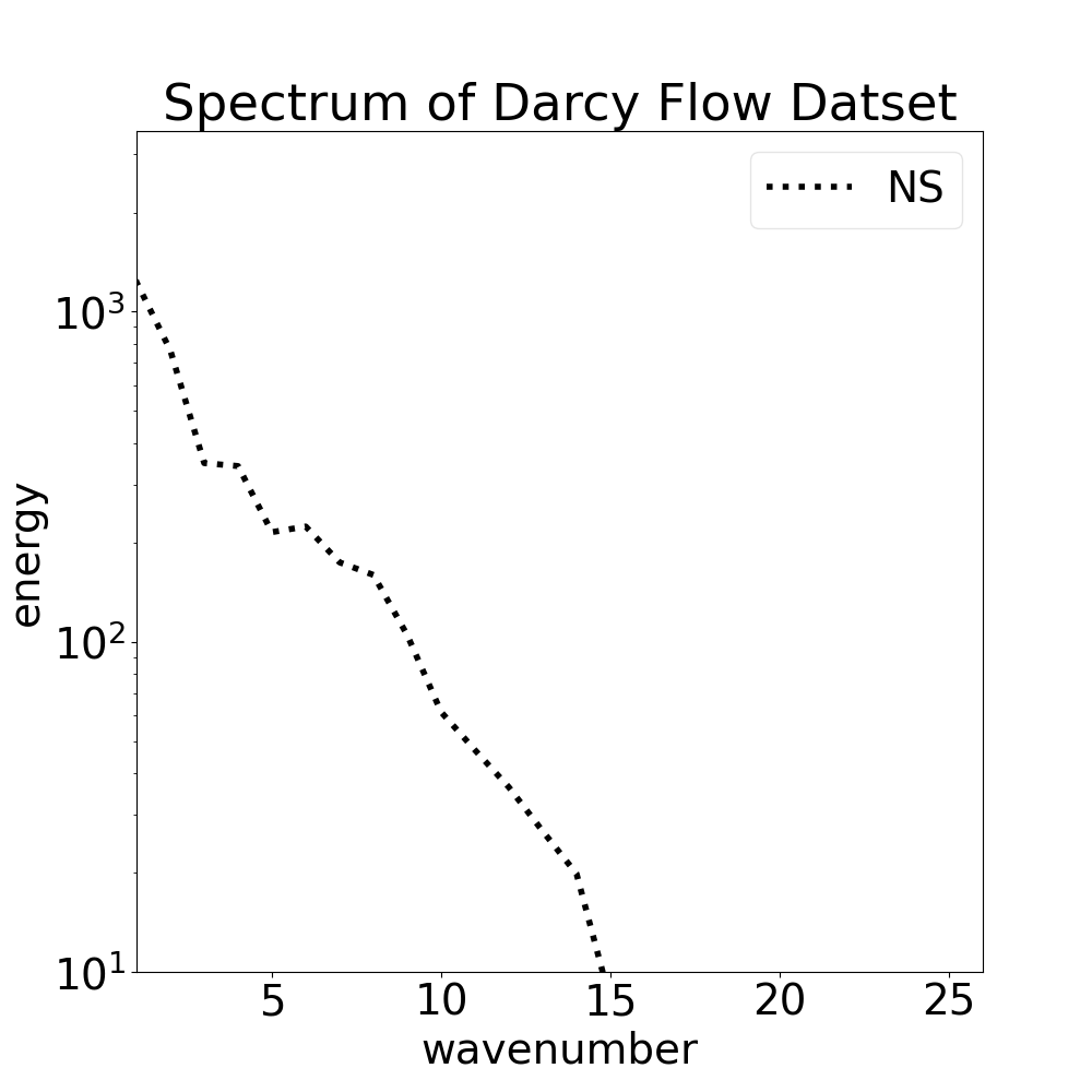
Visualizing the energy spectrum

The energy spectrum shows how much energy is contained in each wavenumber (spatial frequency) Higher wavenumbers correspond to smaller spatial scales and higher frequencies

# Configure pyplot and generate the plot
plt.style.use("classic")
fig, ax = plt.subplots(figsize=(10, 10), dpi=150)
ax.set_facecolor("white")
ax.set_yscale("log")  # Log scale for better visualization of energy decay
length = dataset_pred.shape[-1]  # The resolution length of the dataset
buffer = 4  # Add a buffer to the plot for better visualization
k = np.arange(length + buffer) * 1.0

# Plot the spectrum
ax.plot(truth_sp, color="navy", linestyle="--", linewidth=2.5, label="Energy Spectrum")

# Customizing the plot
ax.set_xlim(1, 16)
ax.set_ylim(0.01, 20)
ax.set_xlabel("Wavenumber", fontsize=16, fontweight="bold")
ax.set_ylabel("Energy", fontsize=16, fontweight="bold")
ax.set_title(
    f"Energy Spectrum of {dataset_name} Dataset", fontsize=18, fontweight="bold", pad=20
)
ax.tick_params(axis="both", which="major", labelsize=15)

plt.tight_layout()
plt.show()

Total running time of the script: (0 minutes 0.810 seconds)

Gallery generated by Sphinx-Gallery