Note
Go to the end to download the full example code.
Training an FNO on Darcy-Flow
We train a Fourier Neural Operator (FNO) on our small Darcy-Flow example.
This tutorial demonstrates the complete workflow of training a neural operator: 1. Loading and preprocessing the Darcy-Flow dataset 2. Creating an FNO model architecture 3. Setting up training components (optimizer, scheduler, losses) 4. Training the model 5. Evaluating predictions and zero-shot super-resolution
Note that this dataset is much smaller than one we would use in practice. The small Darcy-flow is an example built to be trained on a CPU in a few seconds, whereas normally we would train on one or multiple GPUs.
The FNO’s key advantage is its resolution invariance - it can make predictions at different resolutions without retraining, which we will demonstrate in the zero-shot super-resolution section.
Import dependencies
We import the necessary modules from neuralop for training a Fourier Neural Operator
import torch
import matplotlib.pyplot as plt
import sys
from neuralop.models import FNO
from neuralop import Trainer
from neuralop.training import AdamW
from neuralop.data.datasets import load_darcy_flow_small
from neuralop.utils import count_model_params
from neuralop import LpLoss, H1Loss

device = "cpu"
Loading the Darcy-Flow dataset
We load the small Darcy-Flow dataset with multiple resolutions for training and testing. The dataset contains permeability fields (input) and pressure fields (output).
train_loader, test_loaders, data_processor = load_darcy_flow_small(
    n_train=1000,
    batch_size=64,
    n_tests=[100, 50],
    test_resolutions=[16, 32],
    test_batch_sizes=[32, 32],
)
data_processor = data_processor.to(device)
Loading test db for resolution 16 with 100 samples
Loading test db for resolution 32 with 50 samples
Creating the FNO model
model = FNO(
    n_modes=(8, 8),
    in_channels=1,
    out_channels=1,
    hidden_channels=24,
    projection_channel_ratio=2,
)
model = model.to(device)

# Count and display the number of parameters
n_params = count_model_params(model)
print(f"\nOur model has {n_params} parameters.")
sys.stdout.flush()
Our model has 191881 parameters.
Creating the optimizer and scheduler
We use AdamW optimizer with weight decay for regularization
optimizer = AdamW(model.parameters(), lr=1e-2, weight_decay=1e-4)
scheduler = torch.optim.lr_scheduler.CosineAnnealingLR(optimizer, T_max=30)
Setting up loss functions
We use H1 loss for training and L2 loss for evaluation H1 loss is particularly good for PDE problems as it penalizes both function values and gradients
l2loss = LpLoss(d=2, p=2)  # L2 loss for function values
h1loss = H1Loss(d=2)  # H1 loss includes gradient information

train_loss = h1loss
eval_losses = {"h1": h1loss, "l2": l2loss}
Training the model
We display the training configuration and then train the model
print("\n### MODEL ###\n", model)
print("\n### OPTIMIZER ###\n", optimizer)
print("\n### SCHEDULER ###\n", scheduler)
print("\n### LOSSES ###")
print(f"\n * Train: {train_loss}")
print(f"\n * Test: {eval_losses}")
sys.stdout.flush()
### MODEL ###
 FNO(
  (positional_embedding): GridEmbeddingND()
  (fno_blocks): FNOBlocks(
    (convs): ModuleList(
      (0-3): 4 x SpectralConv(
        (weight): DenseTensor(shape=torch.Size([24, 24, 8, 5]), rank=None)
      )
    )
    (fno_skips): ModuleList(
      (0-3): 4 x Flattened1dConv(
        (conv): Conv1d(24, 24, kernel_size=(1,), stride=(1,), bias=False)
      )
    )
    (channel_mlp): ModuleList(
      (0-3): 4 x ChannelMLP(
        (fcs): ModuleList(
          (0): Conv1d(24, 12, kernel_size=(1,), stride=(1,))
          (1): Conv1d(12, 24, kernel_size=(1,), stride=(1,))
        )
      )
    )
    (channel_mlp_skips): ModuleList(
      (0-3): 4 x SoftGating()
    )
  )
  (lifting): ChannelMLP(
    (fcs): ModuleList(
      (0): Conv1d(3, 48, kernel_size=(1,), stride=(1,))
      (1): Conv1d(48, 24, kernel_size=(1,), stride=(1,))
    )
  )
  (projection): ChannelMLP(
    (fcs): ModuleList(
      (0): Conv1d(24, 48, kernel_size=(1,), stride=(1,))
      (1): Conv1d(48, 1, kernel_size=(1,), stride=(1,))
    )
  )
)

### OPTIMIZER ###
 AdamW (
Parameter Group 0
    betas: (0.9, 0.999)
    correct_bias: True
    eps: 1e-06
    initial_lr: 0.01
    lr: 0.01
    weight_decay: 0.0001
)

### SCHEDULER ###
 <torch.optim.lr_scheduler.CosineAnnealingLR object at 0x7fbc973379d0>

### LOSSES ###

 * Train: <neuralop.losses.data_losses.H1Loss object at 0x7fbc97336ad0>

 * Test: {'h1': <neuralop.losses.data_losses.H1Loss object at 0x7fbc97336ad0>, 'l2': <neuralop.losses.data_losses.LpLoss object at 0x7fbc97337b10>}
Creating the trainer
We create a Trainer object that handles the training loop, evaluation, and logging
trainer = Trainer(
    model=model,
    n_epochs=15,
    device=device,
    data_processor=data_processor,
    wandb_log=False,  # Disable Weights & Biases logging for this tutorial
    eval_interval=5,  # Evaluate every 5 epochs
    use_distributed=False,  # Single GPU/CPU training
    verbose=True,  # Print training progress
)
Training the model
We train the model on our Darcy-Flow dataset. The trainer will: 1. Run the forward pass through the FNO 2. Compute the H1 loss 3. Backpropagate and update weights 4. Evaluate on test data every 3 epochs
trainer.train(
    train_loader=train_loader,
    test_loaders=test_loaders,
    optimizer=optimizer,
    scheduler=scheduler,
    regularizer=False,
    training_loss=train_loss,
    eval_losses=eval_losses,
)
Training on 1000 samples
Testing on [50, 50] samples         on resolutions [16, 32].
/opt/hostedtoolcache/Python/3.13.14/x64/lib/python3.13/site-packages/torch/utils/data/dataloader.py:1095: UserWarning: 'pin_memory' argument is set as true but no accelerator is found, then device pinned memory won't be used.
  super().__init__(loader)
/opt/hostedtoolcache/Python/3.13.14/x64/lib/python3.13/site-packages/torch/nn/modules/module.py:1789: UserWarning: FNO.forward() received unexpected keyword arguments: ['y']. These arguments will be ignored.
  return forward_call(*args, **kwargs)
Raw outputs of shape torch.Size([64, 1, 16, 16])
/home/runner/work/neuraloperator/neuraloperator/neuralop/training/trainer.py:536: UserWarning: H1Loss.__call__() received unexpected keyword arguments: ['x']. These arguments will be ignored.
  loss += training_loss(out, **sample)
[0] time=1.13, avg_loss=0.7617, train_err=47.6062
/home/runner/work/neuraloperator/neuraloperator/neuralop/training/trainer.py:581: UserWarning: LpLoss.__call__() received unexpected keyword arguments: ['x']. These arguments will be ignored.
  val_loss = loss(out, **sample)
Eval: 16_h1=0.5218, 16_l2=0.3231, 32_h1=0.6226, 32_l2=0.3236
[5] time=1.09, avg_loss=0.2588, train_err=16.1757
Eval: 16_h1=0.2487, 16_l2=0.1704, 32_h1=0.3766, 32_l2=0.1918
[10] time=1.09, avg_loss=0.1991, train_err=12.4459
Eval: 16_h1=0.2050, 16_l2=0.1331, 32_h1=0.3422, 32_l2=0.1616

{'train_err': 11.168464809656143, 'avg_loss': 0.1786954369544983, 'avg_lasso_loss': None, 'epoch_train_time': 1.0921109439999555}
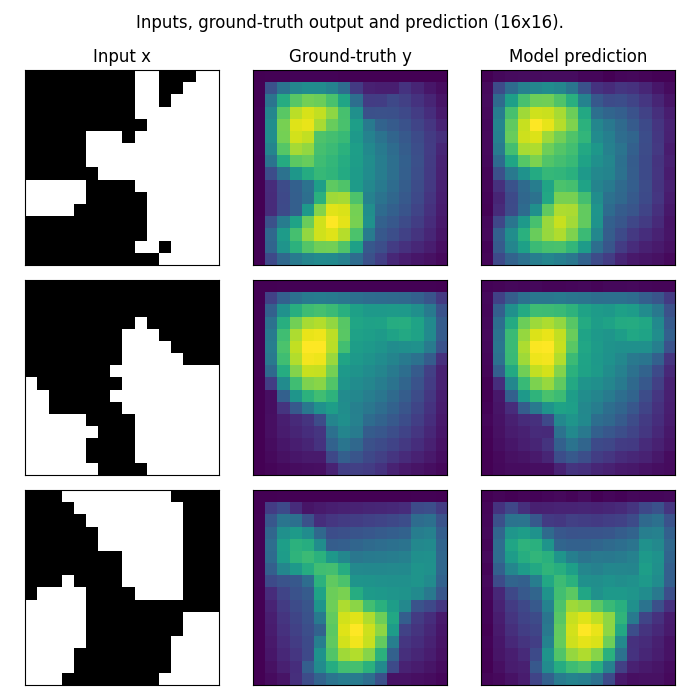
Visualizing predictions
Let’s take a look at what our model’s predicted outputs look like. We wll compare the inputs, ground-truth outputs, and model predictions side by side.
Note that in this example, we train on a very small resolution for a very small number of epochs. In practice, we would train at a larger resolution on many more samples.
test_samples = test_loaders[16].dataset

fig = plt.figure(figsize=(7, 7))
for index in range(3):
    data = test_samples[index]
    data = data_processor.preprocess(data, batched=False)

    # Input
    x = data["x"]
    # Ground-truth output
    y = data["y"]
    # Model prediction
    out = model(x.unsqueeze(0))

    # Plot input
    ax = fig.add_subplot(3, 3, index * 3 + 1)
    ax.imshow(x[0], cmap="gray")
    if index == 0:
        ax.set_title("Input x")
    plt.xticks([], [])
    plt.yticks([], [])

    # Plot ground-truth output
    ax = fig.add_subplot(3, 3, index * 3 + 2)
    ax.imshow(y.squeeze())
    if index == 0:
        ax.set_title("Ground-truth output")
    plt.xticks([], [])
    plt.yticks([], [])

    # Plot model prediction
    ax = fig.add_subplot(3, 3, index * 3 + 3)
    ax.imshow(out.squeeze().detach().numpy())
    if index == 0:
        ax.set_title("Model prediction")
    plt.xticks([], [])
    plt.yticks([], [])

fig.suptitle("FNO predictions on 16x16 Darcy-Flow data", y=0.98)
plt.tight_layout()
fig.show()
Zero-shot super-resolution evaluation
One of the key advantages of neural operators is their resolution invariance. The FNO’s invariance to the discretization of input data means we can natively make predictions on higher-resolution inputs and get higher-resolution outputs without retraining the model!
test_samples = test_loaders[32].dataset

fig = plt.figure(figsize=(7, 7))
for index in range(3):
    data = test_samples[index]
    data = data_processor.preprocess(data, batched=False)

    # Input at higher-resolution
    x = data["x"]
    # Ground-truth output at higher-resolution
    y = data["y"]
    # Model prediction at higher-resolution
    out = model(x.unsqueeze(0))

    # Plot input at higher-resolution
    ax = fig.add_subplot(3, 3, index * 3 + 1)
    ax.imshow(x[0], cmap="gray")
    if index == 0:
        ax.set_title("Input at 32x32")
    plt.xticks([], [])
    plt.yticks([], [])

    # Plot ground-truth output at higher-resolution
    ax = fig.add_subplot(3, 3, index * 3 + 2)
    ax.imshow(y.squeeze())
    if index == 0:
        ax.set_title("Ground-truth at 32x32")
    plt.xticks([], [])
    plt.yticks([], [])

    # Plot model prediction at higher-resolution
    ax = fig.add_subplot(3, 3, index * 3 + 3)
    ax.imshow(out.squeeze().detach().numpy())
    if index == 0:
        ax.set_title("FNO prediction at 32x32")
    plt.xticks([], [])
    plt.yticks([], [])

fig.suptitle("Zero-shot super-resolution: 16x16 → 32x32", y=0.98)
plt.tight_layout()
fig.show()
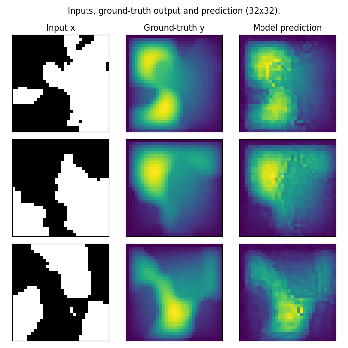
Understanding zero-shot super-resolution
We only trained the model on data at a resolution of 16x16, and with no modifications or special prompting, we were able to perform inference on higher-resolution input data and get higher-resolution predictions! This is a powerful capability of neural operators.
In practice, we often want to evaluate neural operators at multiple resolutions to track a model’s zero-shot super-resolution performance throughout training. That’s why many of our datasets, including the small Darcy-flow we showcased, are parameterized with a list of test_resolutions to choose from.
Note: These predictions may be noisier than we would expect for a model evaluated at the same resolution at which it was trained. This is because the model hasn’t seen the higher-frequency patterns present in the 32x32 data during training. However, this demonstrates the fundamental resolution invariance of neural operators.
Total running time of the script: (0 minutes 17.489 seconds)