Neural Operators: an Introduction
This guide introduces neural operators, a class of models that learn mappings between function spaces and solve partial differential equations. You can also check out the papers [1] [2] [3] [4] for more details.
Introduction
Scientific computations are often very costly in terms of time and resources. For example, running numerical simulations of fluid dynamics or many-body systems can take days or even months. This high cost is largely due to the need for numerical solvers to discretize space and time into extremely fine grids in order to achieve acceptable accuracy. Solving the resulting large number of equations on these grids is computationally intensive.
To address these challenges, researchers have started to develop data-driven approaches using machine learning. Rather than explicitly solving the equations for each new scenario, data-driven solvers are trained on data that pairs problems with their solutions. Once trained, these solvers can quickly make predictions for new problems based on input data. Because they do not require breaking the domain into tiny pieces and solving every equation from scratch, data-driven methods are often much faster than traditional numerical solvers.
However, data-driven solvers are subject to the quality of the input and training data. If the training data is not good enough, they will learn to emulate that unreliable data and will not make good predictions. In scientific computing, usually, the training data are generated by traditional numerical solvers, and it can still take days or months for these numerical solvers to generate good enough data. In some cases, data are gathered directly from experiments, and high-quality training data may be unavailable.
Neural networks are often regarded as powerful interpolators, but their ability to extrapolate to unseen scenarios remains uncertain. This raises questions about their capacity to generalize beyond the specific conditions represented in the training data. For example, if training data are generated at a particular resolution, the resulting learned models may only work effectively at that resolution. Overall, generalization is a fundamental challenge in machine learning. As a result, while machine learning-based methods can significantly speed up evaluation, the process of obtaining and preparing suitable training data can remain time-consuming and difficult.
To address this challenge, we introduce operator learning. By encoding appropriate structures, we enable neural networks to learn mappings between functions and to generalize across different discretizations. This means we can use numerical methods to generate less-accurate, low-resolution data, yet the trained solver can still produce accurate, high-resolution predictions. As a result, both training and evaluation can become significantly more efficient and straightforward.
Operator Learning
In mathematics, the term “operator” commonly refers to a mapping between function spaces. You have likely encountered familiar operators such as differentiation and integration. Applying a derivative or performing an indefinite integration on a function transforms it into another function, which are both classic examples of operators acting on function spaces.
In scientific computing, the core challenge often involves solving differential equations, which inherently relate operators to function spaces. Consider a general differential equation of the form:
where \(u\) and \(f\) are some functions on the physical domain, and \(\mathcal{L}\) is some differential operator that maps the function \(u\) to the function \(f\). In most cases, \(\mathcal{L}\) and \(f\) are specified, and the objective is to find the solution \(u\). Viewed from this perspective, solving a PDE is fundamentally an operator learning task: we wish to learn the mapping from input functions to solution functions.
Traditionally, neural networks have been designed to model mappings between finite-dimensional Euclidean spaces, such as classifying an image (represented as a vector of pixel intensities) into a label, or transforming one image vector into another. While effective for many tasks, this framework is inherently limited when addressing scientific and mathematical problems that require learning mappings between entire function spaces. In these cases, rather than learning simple vector-to-vector transformations, we seek to learn operators: transformations that act on functions and produce new functions, which is a more complex and general task.
This challenge is not restricted to the domain of differential equations; operator learning is implicit in many machine learning applications. For instance, even images can be more accurately viewed as continuous functions of light intensity over a spatial domain, rather than as discrete \(32 \times 32\) pixel arrays. By embracing this perspective, we gain the flexibility to reason about, and learn mappings between, functions defined on arbitrary continuous domains, transcending the constraints of fixed discretizations.
We discuss how to generalize neural networks so that they can learn operators, the mappings between infinite-dimensional spaces, with a special focus on PDEs. For a comprehensive guide on principled approaches for extending neural architectures to function spaces for operator learning, see [3].
Limitation of Fixed Discretization
Solving partial differential equations (PDEs) is a notoriously challenging task. Rather than working directly with operators on infinite-dimensional function spaces, the standard approach is to discretize the physical domain and reformulate the problem in a finite-dimensional Euclidean setting. Over the past century, this has led to the development of powerful numerical methods, such as the finite element method and the finite difference method, which remain the cornerstone tools for PDE solution.
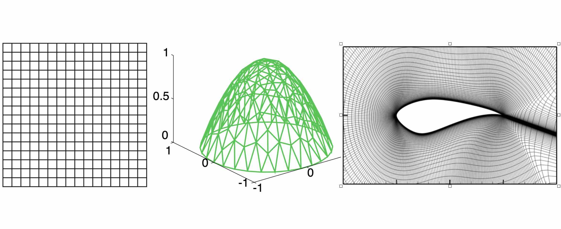
Three examples of discretization: The left one is a regular grid used in the finite difference method; the middle one is a triangulated grid used in the finite element method; the right one is a cylinder mesh for real-world airfoil problem.
Just like how we store images by pixels in .PNG and .JPG formats, we need to discretize the domain of PDEs into some grid and solve the equation on the grid. It really makes the thing easier. These traditional numerical solvers are awesome, but they have some drawbacks:
The error scales steeply with the resolution, so we often need a high resolution to get good approximations.
The computation and storage steeply scale with the resolution (i.e. the size of the grid).
When the equation is solved on one discretization, we cannot change the discretization anymore.
While formats like .PNG and .JPG are well-suited for storing images as grids of pixels, sometimes it’s advantageous to use vector formats such as .EPS or .SVG, which represent images in a resolution-independent way and can be scaled or manipulated flexibly. For certain types of images, vector formats can be both more convenient and more efficient.
In the same spirit, when dealing with PDEs, we seek a representation that is not tied to any particular discretization, in other words, a continuous formulation of the problem. This means learning an operator that acts on functions directly and is invariant to the discretization, much like how a vector image can be displayed on any device at any resolution.
From a mathematical perspective, a continuous, discretization-invariant representation aligns more closely with the true analytic solution of a problem. This approach is not only conceptually elegant but also carries significant theoretical meaning. Keeping this motivation in mind, let us now build a rigorous mathematical framework.
Problem Setting
Consider the standard second order elliptic PDE
for some bounded, open domain \(D \subset \mathbb{R}^d\) and a fixed source function \(f\). This equation is prototypical of PDEs arising in numerous applications including hydrology and elasticity. For a given function \(a\), the equation has a unique weak solution \(u\) and therefore we can define the solution operator \(\mathcal{F}_{true}\) as the map from function to function \(a \mapsto u\).
Our goal is to learn a operator \(\mathcal{F}\) approximating \(\mathcal{F}_{true}\), by using a finite collection of observations of input-output pairs \(\{a_j, u_j\}_{j=1}^N\), where each \(a_j\) and \(u_j\) are functions on \(D\). In practice, the training data is solved numerically or observed in experiments. In other words, functions \(a_j\) and \(u_j\) come with discretization. Let \(P_K = \{x_1,\dots,x_K\} \subset D\) be a \(K\)-point discretization of the domain \(D\) and assume we have observations \(a_j|_{P_K}, u_j|_{P_K}\), for a finite collection of input-output pairs indexed by \(j\).
We will show how to learn a discretization-invariant mapping based on discretized data.
Kernel Formulation
For a general PDE of the form:
Under fairly general conditions on \(\mathcal{L}_a\), we may define the Green’s function \(G : D \times D \to \mathbb{R}\) as the unique solution to the problem
where \(\delta_x\) is the delta measure on \(\mathbb{R}^d\) centered at \(x\). Note that \(G\) will depend on the coefficient \(a\) thus we will henceforth denote it as \(G_a\). Then the true operator \(\mathcal{F}_{true}\) can be written as an integral operator of Green’s function:
Generally, the Green’s function is continuous at points \(x \neq y\), for example, when \(\mathcal{L}_a\) is uniformly elliptic. Hence it is natural to model the kernel via a neural network \(\kappa\). Just as the Green’s function, the kernel network \(\kappa\) takes input \((x,y)\). Since the kernel depends on \(a\), we let \(\kappa\) also take input \((a(x),a(y))\), i.e.
As an Iterative Solver
In our setting, \(f\) is an unknown but fixed function. Instead of performing the kernel convolution with \(f\), we will formulate it as an iterative solver that approximates \(u\) via \(u_t\), where \(t = 0,\ldots,T\) is the time step.
The algorithm starts from an initialization \(u_0\), for which we use \(u_0(x) = (x, a(x))\). At each time step \(t\), it updates \(u_{t+1}\) via a kernel convolution of \(u_{t}\), i.e.
It works like an implicit iteration, where at each iteration the algorithm solves an equation for \(u_{t}(x)\) and \(u_{t+1}(x)\) using the kernel integral. \(u_T\) will be output as the final prediction.
To further take the advantage of neural networks, we will lift \(u(x) \in \mathbb{R}^d\) to a high dimensional representation \(v(x) \in \mathbb{R}^n\), with \(n\) the dimension of the hidden representation.
The overall algorithmic framework follow:
where \(NN_1\) and \(NN_2\) are two feed-forward neural networks that lifts the initialization to hidden representation \(v\) and projects the representation back to the solution \(u\), respectively. \(\sigma\) is an activation function such as ReLU. The additional term \(W \in \mathbb{R}^{n \times n}\) is a linear transformation that acts on \(v\).
Notice that since the kernel integration happens in the high dimensional representation, the output of \(\kappa_{\phi}\) is not a scalar, but a linear transformation \(\kappa_{\phi}\big(x,y,a(x),a(y)\big)\in \mathbb{R}^{n \times n}\).
Graph Neural Networks
To perform the integration, we again need some discretization. Assuming a uniform distribution of \(y\), the integral \(\int_{B(x,r)} \kappa_{\phi}\big(x,y,a(x),a(y)\big) v_t(y)\: \mathrm{d}y\) can be approximated by a sum:
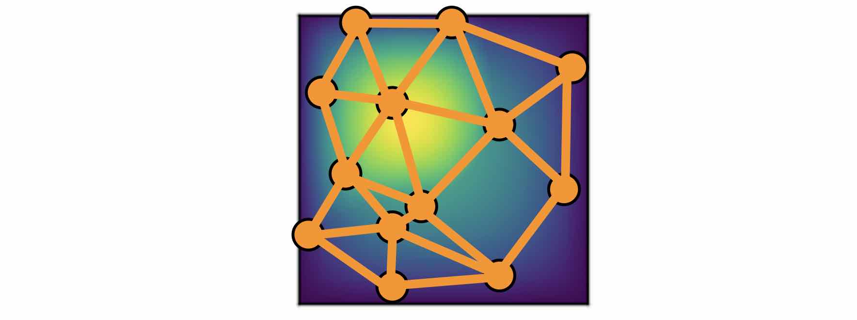
Observation: The kernel integral is equivalent to message passing on graphs.
If you are familiar with graph neural networks, you may have already realized this formulation is the same as the aggregation of messages in graph networks. Message passing graph networks comprise a standard architecture employing edge features (Gilmer et al, 2017).
If we properly construct graphs on the spatial domain \(D\) of the PDE, the kernel integration can be viewed as an aggregation of messages. Given node features \(v_t(x) \in \mathbb{R}^{n}\), edge features \(e(x,y) \in \mathbb{R}^{n_e}\), and a graph \(G\), the message passing neural network with averaging aggregation is
where \(W \in \mathbb{R}^{n \times n}\), \(N(x)\) is the neighborhood of \(x\) according to the graph, \(\kappa_{\phi}\big(e(x,y)\big)\) is a neural network taking edge features as input and as output a matrix in \(\mathbb{R}^{n \times n}\). Relating to our kernel formulation, \(e(x,y) = (x,y,a(x),a(y))\).
Nystrom Approximation
Ideally, to use all the information available, we should construct \(K\) nodes in the graph for all the points in the discretization \(P_k = \{x_1,\ldots, x_K\}\), which will create \(O(K^2)\) edges. It is quite expensive. Thankfully, we don’t need all the points to get an accurate approximation. For each graph, the error of Monte Carlo approximation of the kernel integral
scales with \(m^{-1/2}\), where \(m\) is the number of nodes sampled.
Since we will sample \(N\) graphs in total for all \(N\) training examples \(\{a_j, u_j\}^N\), the overall error of the kernel is much smaller than \(m^{-1/2}\), where \(m\) is the number of nodes sampled. In practice, sampling \(m \sim 200\) nodes is sufficient for \(K \sim 100,\!000\) points.
The approximation can be further improved by employing advanced Nystrom methods. For instance, by estimating the significance or influence of each point, we can strategically allocate more nodes to regions with high complexity or singularities in the PDEs, leading to greater accuracy where it matters most.
Experiments: Poisson Equations
Let’s first consider a simple Poisson equation:
We set \(v_0 = f\) and \(T=1\), and use one iteration of the graph kernel network to learn the operator \(\mathcal{F}: f \mapsto u\).
Poisson equation
As shown in the figure above, we compare the true analytic Green’s function \(G(x,y)\) (left) with the learned kernel \(\kappa_{\phi}(x,y)\) (right). The learned kernel is almost the same as the true kernel, which means our neural network formulation matches the Green’s function expression.
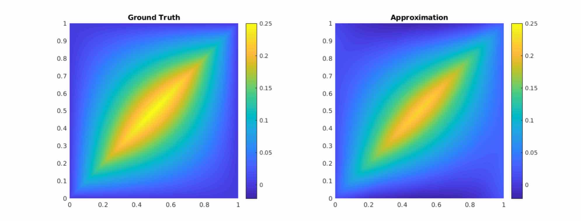
2D Poisson equation
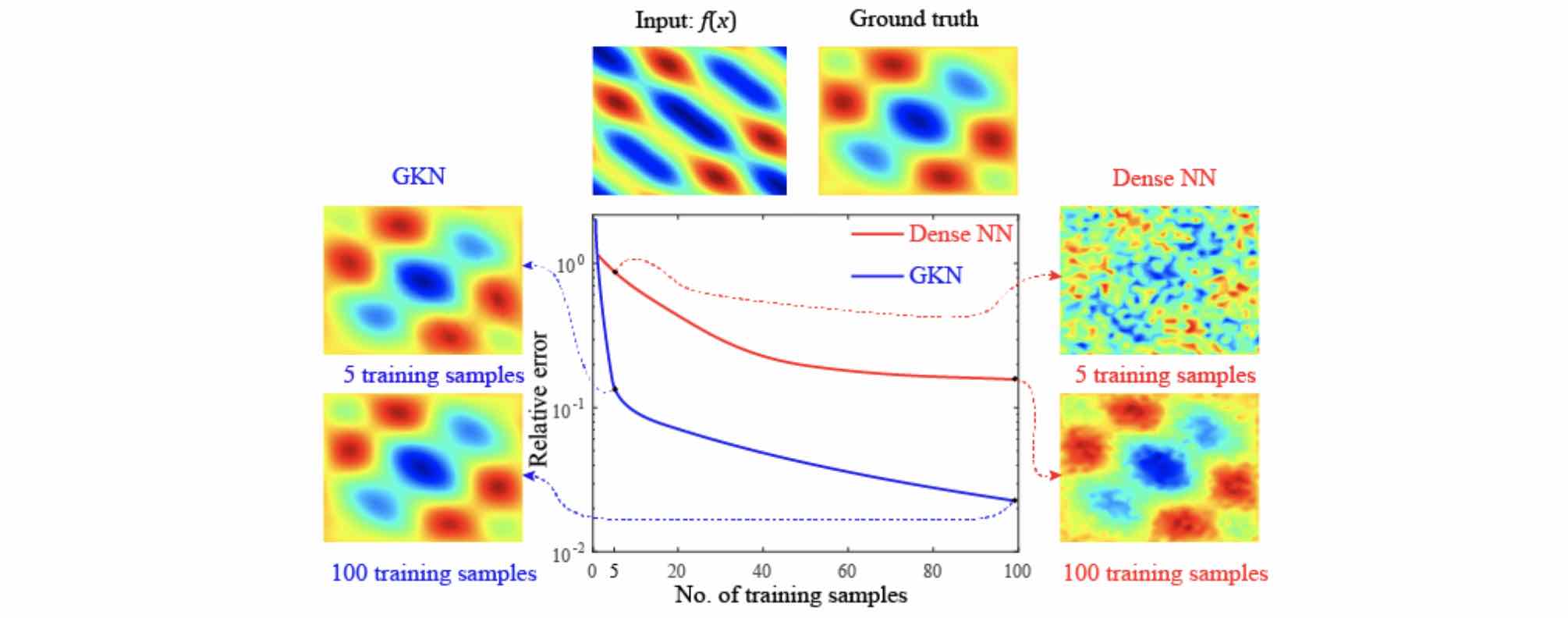
By assuming the kernel structure, graph kernel networks need only a few training examples to learn the shape of the solution \(u\). As shown in the figure above, the graph kernel network can roughly learn \(u\) with \(5\) training pairs, while a feedforward neural network needs at least \(100\) training examples.
Experiments: generalization of resolution
For the large scale experiments, we use the Darcy equation of the form
and learn the operator \(\mathcal{F}: a \mapsto u\).
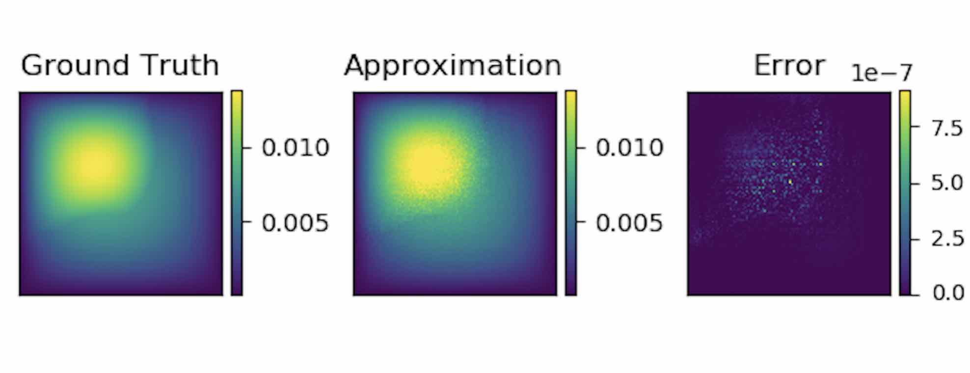
To demonstrate the generalization property, we train the graph kernel network with nodes sampled from the resolution \(s \times s\) and test on a different resolution \(s' \times s'\) .
As shown in the table above for each row, the test errors on different resolutions are about the same, which means the graph kernel network can also generalize in the semi-supervised setting. A figure for \(s=16, s'=241\) is shown below (where the error is the absolute squared error):
Conclusion
We proposed using graph networks for operator learning in PDE problems. By varying the underlying graph and discretization, the learned kernel is invariant to the discretization. Experiments confirm that the graph kernel networks are able to generalize among different discretizations. And in the fixed discretization setting, the graph kernel networks also have good performance compared to several benchmarks.