Note
Go to the end to download the full example code.
Training an FNO with incremental meta-learning
A demo of the Incremental FNO meta-learning algorithm on our small Darcy-Flow dataset.
This tutorial demonstrates incremental meta-learning for neural operators, which allows the model to gradually increase its complexity during training. This approach can lead to:
Better convergence properties
More stable training dynamics
Improved generalization
Reduced computational requirements during early training
The incremental approach starts with a small number of Fourier modes and gradually increases the model capacity as training progresses.
Import dependencies
We import the necessary modules for incremental FNO training
import torch
import matplotlib.pyplot as plt
import sys
from neuralop.models import FNO
from neuralop.data.datasets import load_darcy_flow_small
from neuralop.utils import count_model_params
from neuralop.training import AdamW
from neuralop.training.incremental import IncrementalFNOTrainer
from neuralop.data.transforms.data_processors import IncrementalDataProcessor
from neuralop import LpLoss, H1Loss
Loading the Darcy-Flow dataset
We load the Darcy-Flow dataset with multiple resolutions for incremental training.
train_loader, test_loaders, output_encoder = load_darcy_flow_small(
    n_train=100,
    batch_size=16,
    test_resolutions=[16, 32],
    n_tests=[100, 50],
    test_batch_sizes=[32, 32],
)

device = torch.device("cuda" if torch.cuda.is_available() else "cpu")
Loading test db for resolution 16 with 100 samples
Loading test db for resolution 32 with 50 samples
Configuring incremental training
We set up the incremental FNO model with a small starting number of modes. The model will gradually increase its capacity during training. We choose to update the modes using the incremental gradient explained algorithm
incremental = True
if incremental:
    starting_modes = (2, 2)  # Start with very few modes
else:
    starting_modes = (8, 8)  # Standard number of modes
Creating the incremental FNO model
We create an FNO model with a maximum number of modes that can be reached during incremental training. The model starts with fewer modes and grows.
model = FNO(
    max_n_modes=(8, 8),  # Maximum modes the model can reach
    n_modes=starting_modes,  # Starting number of modes
    hidden_channels=32,
    in_channels=1,
    out_channels=1,
)
model = model.to(device)
n_params = count_model_params(model)
Setting up the optimizer and scheduler
We use AdamW optimizer with weight decay for regularization
optimizer = AdamW(model.parameters(), lr=8e-3, weight_decay=1e-4)
scheduler = torch.optim.lr_scheduler.CosineAnnealingLR(optimizer, T_max=30)
Configuring incremental data processing
If one wants to use Incremental Resolution, one should use the IncrementalDataProcessor. When passed to the trainer, the trainer will automatically update the resolution.
Key parameters for incremental resolution:
incremental_resolution: bool, default is False. If True, increase the resolution of the input incrementally
incremental_res_gap: parameter for resolution updates
subsampling_rates: a list of resolutions to use
dataset_indices: a list of indices of the dataset to slice to regularize the input resolution
dataset_resolution: the resolution of the input
epoch_gap: the number of epochs to wait before increasing the resolution
verbose: if True, print the resolution and the number of modes
data_transform = IncrementalDataProcessor(
    in_normalizer=None,
    out_normalizer=None,
    device=device,
    subsampling_rates=[2, 1],  # Resolution scaling factors
    dataset_resolution=16,  # Base resolution
    dataset_indices=[2, 3],  # Dataset indices for regularization
    epoch_gap=10,  # Epochs between resolution updates
    verbose=True,  # Print progress information
)

data_transform = data_transform.to(device)
Original Incre Res: change index to 0
Original Incre Res: change sub to 2
Original Incre Res: change res to 8
Setting up loss functions
We use H1 loss for training and L2 loss for evaluation
l2loss = LpLoss(d=2, p=2)
h1loss = H1Loss(d=2)
train_loss = h1loss
eval_losses = {"h1": h1loss, "l2": l2loss}
Displaying training configuration
We display the model parameters, optimizer, scheduler, and loss functions to verify our incremental training setup
print("\n### N PARAMS ###\n", n_params)
print("\n### OPTIMIZER ###\n", optimizer)
print("\n### SCHEDULER ###\n", scheduler)
print("\n### LOSSES ###")
print("\n### INCREMENTAL RESOLUTION + GRADIENT EXPLAINED ###")
print(f"\n * Train: {train_loss}")
print(f"\n * Test: {eval_losses}")
sys.stdout.flush()
### N PARAMS ###
 537441

### OPTIMIZER ###
 AdamW (
Parameter Group 0
    betas: (0.9, 0.999)
    correct_bias: True
    eps: 1e-06
    initial_lr: 0.008
    lr: 0.008
    weight_decay: 0.0001
)

### SCHEDULER ###
 <torch.optim.lr_scheduler.CosineAnnealingLR object at 0x7fbc8417e650>

### LOSSES ###

### INCREMENTAL RESOLUTION + GRADIENT EXPLAINED ###

 * Train: <neuralop.losses.data_losses.H1Loss object at 0x7fbc7516d090>

 * Test: {'h1': <neuralop.losses.data_losses.H1Loss object at 0x7fbc7516d090>, 'l2': <neuralop.losses.data_losses.LpLoss object at 0x7fbc8417e2c0>}
Configuring the IncrementalFNOTrainer
We set up the IncrementalFNOTrainer with various incremental learning options. Other options include setting incremental_loss_gap = True. If one wants to use incremental resolution, set it to True. In this example we only update the modes and not the resolution. When using incremental resolution, keep in mind that the number of modes initially set should be strictly less than the resolution.
Key parameters for incremental training:
incremental_grad: bool, default is False. If True, use the base incremental algorithm based on gradient variance
incremental_grad_eps: threshold for gradient variance
incremental_buffer: number of buffer modes to calculate gradient variance
incremental_max_iter: initial number of iterations
incremental_grad_max_iter: maximum iterations to accumulate gradients
incremental_loss_gap: bool, default is False. If True, use the incremental algorithm based on loss gap
incremental_loss_eps: threshold for loss gap
# Create the IncrementalFNOTrainer with our configuration
trainer = IncrementalFNOTrainer(
    model=model,
    n_epochs=20,
    data_processor=data_transform,
    device=device,
    verbose=True,
    incremental_loss_gap=False,  # Use gradient-based incremental learning
    incremental_grad=True,  # Enable gradient-based mode updates
    incremental_grad_eps=0.9999,  # Gradient variance threshold
    incremental_loss_eps=0.001,  # Loss gap threshold
    incremental_buffer=5,  # Buffer modes for gradient calculation
    incremental_max_iter=1,  # Initial iterations
    incremental_grad_max_iter=2,  # Maximum gradient accumulation iterations
)
Training the incremental FNO model
We train the model using incremental meta-learning. The trainer will: 1. Start with a small number of Fourier modes 2. Gradually increase the model capacity based on gradient variance 3. Monitor the incremental learning progress 4. Evaluate on test data throughout training
trainer.train(
    train_loader,
    test_loaders,
    optimizer,
    scheduler,
    regularizer=False,
    training_loss=train_loss,
    eval_losses=eval_losses,
)
Training on 100 samples
Testing on [50, 50] samples         on resolutions [16, 32].
/opt/hostedtoolcache/Python/3.13.14/x64/lib/python3.13/site-packages/torch/utils/data/dataloader.py:1095: UserWarning: 'pin_memory' argument is set as true but no accelerator is found, then device pinned memory won't be used.
  super().__init__(loader)
/opt/hostedtoolcache/Python/3.13.14/x64/lib/python3.13/site-packages/torch/nn/modules/module.py:1789: UserWarning: FNO.forward() received unexpected keyword arguments: ['y']. These arguments will be ignored.
  return forward_call(*args, **kwargs)
Raw outputs of shape torch.Size([16, 1, 8, 8])
/home/runner/work/neuraloperator/neuraloperator/neuralop/training/trainer.py:536: UserWarning: H1Loss.__call__() received unexpected keyword arguments: ['x']. These arguments will be ignored.
  loss += training_loss(out, **sample)
[0] time=0.25, avg_loss=0.9304, train_err=13.2921
/home/runner/work/neuraloperator/neuraloperator/neuralop/training/trainer.py:581: UserWarning: LpLoss.__call__() received unexpected keyword arguments: ['x']. These arguments will be ignored.
  val_loss = loss(out, **sample)
Eval: 16_h1=0.8721, 16_l2=0.6645, 32_h1=0.9786, 32_l2=0.6792
[1] time=0.23, avg_loss=0.7344, train_err=10.4912
Eval: 16_h1=0.7733, 16_l2=0.4229, 32_h1=0.9898, 32_l2=0.4441
[2] time=0.23, avg_loss=0.6269, train_err=8.9551
/home/runner/work/neuraloperator/neuraloperator/neuralop/training/incremental.py:244: UserWarning: Converting a tensor with requires_grad=True to a scalar may lead to unexpected behavior.
Consider using tensor.detach() first. (Triggered internally at /pytorch/torch/csrc/autograd/generated/python_variable_methods.cpp:838.)
  torch.Tensor(strength_vector),
Eval: 16_h1=0.8184, 16_l2=0.4816, 32_h1=0.9968, 32_l2=0.5036
[3] time=0.23, avg_loss=0.6245, train_err=8.9212
Eval: 16_h1=0.7108, 16_l2=0.3728, 32_h1=0.8679, 32_l2=0.3919
[4] time=0.23, avg_loss=0.5684, train_err=8.1204
Eval: 16_h1=0.8178, 16_l2=0.4753, 32_h1=1.1135, 32_l2=0.5132
[5] time=0.23, avg_loss=0.5520, train_err=7.8863
Eval: 16_h1=0.7876, 16_l2=0.4661, 32_h1=1.0540, 32_l2=0.4857
[6] time=0.23, avg_loss=0.5694, train_err=8.1350
Eval: 16_h1=0.7870, 16_l2=0.4602, 32_h1=1.1319, 32_l2=0.5039
[7] time=0.23, avg_loss=0.4907, train_err=7.0101
Eval: 16_h1=0.6249, 16_l2=0.3236, 32_h1=0.8469, 32_l2=0.3518
[8] time=0.23, avg_loss=0.4256, train_err=6.0796
Eval: 16_h1=0.7237, 16_l2=0.4238, 32_h1=0.9182, 32_l2=0.4555
[9] time=0.23, avg_loss=0.4811, train_err=6.8729
Eval: 16_h1=0.5829, 16_l2=0.3504, 32_h1=0.8236, 32_l2=0.3849
Incre Res Update: change index to 1
Incre Res Update: change sub to 1
Incre Res Update: change res to 16
[10] time=0.31, avg_loss=0.5237, train_err=7.4809
Eval: 16_h1=0.5012, 16_l2=0.2913, 32_h1=0.6084, 32_l2=0.2829
[11] time=0.30, avg_loss=0.4472, train_err=6.3879
Eval: 16_h1=0.5117, 16_l2=0.3063, 32_h1=0.6778, 32_l2=0.3257
[12] time=0.30, avg_loss=0.4627, train_err=6.6098
Eval: 16_h1=0.4777, 16_l2=0.2868, 32_h1=0.6316, 32_l2=0.2877
[13] time=0.30, avg_loss=0.4132, train_err=5.9028
Eval: 16_h1=0.4291, 16_l2=0.2652, 32_h1=0.5632, 32_l2=0.2735
[14] time=0.30, avg_loss=0.3869, train_err=5.5269
Eval: 16_h1=0.4190, 16_l2=0.2472, 32_h1=0.5287, 32_l2=0.2527
[15] time=0.30, avg_loss=0.3951, train_err=5.6450
Eval: 16_h1=0.3830, 16_l2=0.2399, 32_h1=0.5248, 32_l2=0.2600
[16] time=0.30, avg_loss=0.3452, train_err=4.9310
Eval: 16_h1=0.3463, 16_l2=0.2178, 32_h1=0.4691, 32_l2=0.2275
[17] time=0.30, avg_loss=0.3202, train_err=4.5746
Eval: 16_h1=0.4641, 16_l2=0.2897, 32_h1=0.6054, 32_l2=0.2965
[18] time=0.30, avg_loss=0.3974, train_err=5.6767
Eval: 16_h1=0.3880, 16_l2=0.2649, 32_h1=0.4860, 32_l2=0.2759
[19] time=0.30, avg_loss=0.3456, train_err=4.9377
Eval: 16_h1=0.3415, 16_l2=0.2211, 32_h1=0.4778, 32_l2=0.2343

{'train_err': 4.937735336167472, 'avg_loss': 0.34564147353172303, 'avg_lasso_loss': None, 'epoch_train_time': 0.29854820299999574, '16_h1': tensor(0.3415), '16_l2': tensor(0.2211), '32_h1': tensor(0.4778), '32_l2': tensor(0.2343)}
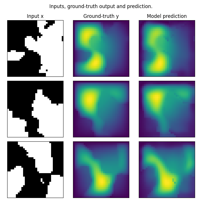
Visualizing incremental FNO predictions
We visualize the model’s predictions after incremental training. Note that we trained on a very small resolution for a very small number of epochs. In practice, we would train at larger resolution on many more samples.
However, for practicality, we created a minimal example that: i) fits in just a few MB of memory ii) can be trained quickly on CPU
In practice we would train a Neural Operator on one or multiple GPUs
test_samples = test_loaders[32].dataset

fig = plt.figure(figsize=(7, 7))
for index in range(3):
    data = test_samples[index]
    # Input x
    x = data["x"].to(device)
    # Ground-truth
    y = data["y"].to(device)
    # Model prediction: incremental FNO output
    out = model(x.unsqueeze(0))

    # Plot input x
    ax = fig.add_subplot(3, 3, index * 3 + 1)
    x = x.cpu().squeeze().detach().numpy()
    y = y.cpu().squeeze().detach().numpy()
    ax.imshow(x, cmap="gray")
    if index == 0:
        ax.set_title("Input x")
    plt.xticks([], [])
    plt.yticks([], [])

    # Plot ground-truth y
    ax = fig.add_subplot(3, 3, index * 3 + 2)
    ax.imshow(y.squeeze())
    if index == 0:
        ax.set_title("Ground-truth y")
    plt.xticks([], [])
    plt.yticks([], [])

    # Plot model prediction
    ax = fig.add_subplot(3, 3, index * 3 + 3)
    ax.imshow(out.cpu().squeeze().detach().numpy())
    if index == 0:
        ax.set_title("Incremental FNO prediction")
    plt.xticks([], [])
    plt.yticks([], [])

fig.suptitle("Incremental FNO predictions on Darcy-Flow data", y=0.98)
plt.tight_layout()
fig.show()
Total running time of the script: (0 minutes 10.951 seconds)