Note
Go to the end to download the full example code.
Training a SFNO on the spherical Shallow Water equations
Using the small Spherical Shallow Water Equations example we ship with the package to train a Spherical Fourier-Neural Operator (SFNO).
This tutorial demonstrates how to train neural operators on spherical domains, which is crucial for many geophysical applications like weather prediction, ocean modeling, and climate science. The SFNO extends the FNO architecture to handle data on the sphere using spherical harmonics instead of regular Fourier modes.
The Shallow Water Equations describe the motion of a thin layer of fluid and are fundamental in atmospheric and oceanic dynamics.
Import dependencies
We import the necessary modules for training a Spherical Fourier Neural Operator
import torch
import matplotlib.pyplot as plt
import sys
from neuralop.models import SFNO
from neuralop import Trainer
from neuralop.training import AdamW
from neuralop.data.datasets import load_spherical_swe
from neuralop.utils import count_model_params
from neuralop import LpLoss, H1Loss

device = torch.device('cuda:0' if torch.cuda.is_available() else 'cpu')
Loading the Spherical Shallow Water Equations dataset
We load the spherical shallow water equations dataset with multiple resolutions. The dataset contains velocity and height fields on the sphere, which are the fundamental variables in shallow water dynamics.
train_loader, test_loaders = load_spherical_swe(n_train=200, batch_size=4, train_resolution=(32, 64),
                                                test_resolutions=[(32, 64), (64, 128)], n_tests=[50, 50], test_batch_sizes=[10, 10],)
Loading train dataloader at resolution (32, 64) with 200 samples and batch-size=4
Loading test dataloader at resolution (32, 64) with 50 samples and batch-size=10
Loading test dataloader at resolution (64, 128) with 50 samples and batch-size=10
Creating the Spherical FNO model
model = SFNO(n_modes=(32, 32),
             in_channels=3,
             out_channels=3,
             hidden_channels=32,
             projection_channel_ratio=2,
             factorization='dense')
model = model.to(device)

# Count and display the number of parameters
n_params = count_model_params(model)
print(f'\nOur model has {n_params} parameters.')
sys.stdout.flush()
Our model has 275555 parameters.
Creating the optimizer and scheduler
We use AdamW optimizer with a lower learning rate for spherical data
optimizer = AdamW(model.parameters(),
                                lr=8e-4,
                                weight_decay=0.0)
scheduler = torch.optim.lr_scheduler.CosineAnnealingLR(optimizer, T_max=30)
Setting up loss functions
For spherical data, we use L2 loss with sum reduction to handle the varying grid sizes across different latitudes on the sphere
l2loss = LpLoss(d=2, p=2, reduction='sum')

train_loss = l2loss
eval_losses={'l2': l2loss}
print('\n### MODEL ###\n', model)
print('\n### OPTIMIZER ###\n', optimizer)
print('\n### SCHEDULER ###\n', scheduler)
print('\n### LOSSES ###')
print(f'\n * Train: {train_loss}')
print(f'\n * Test: {eval_losses}')
sys.stdout.flush()
### MODEL ###
 SFNO(
  (positional_embedding): GridEmbeddingND()
  (fno_blocks): FNOBlocks(
    (convs): ModuleList(
      (0-3): 4 x SphericalConv(
        (weight): ComplexDenseTensor(shape=torch.Size([32, 32, 32]), rank=None)
        (sht_handle): SHT(
          (_SHT_cache): ModuleDict()
          (_iSHT_cache): ModuleDict()
        )
      )
    )
    (fno_skips): ModuleList(
      (0-3): 4 x Flattened1dConv(
        (conv): Conv1d(32, 32, kernel_size=(1,), stride=(1,), bias=False)
      )
    )
    (channel_mlp): ModuleList(
      (0-3): 4 x ChannelMLP(
        (fcs): ModuleList(
          (0): Conv1d(32, 16, kernel_size=(1,), stride=(1,))
          (1): Conv1d(16, 32, kernel_size=(1,), stride=(1,))
        )
      )
    )
    (channel_mlp_skips): ModuleList(
      (0-3): 4 x SoftGating()
    )
  )
  (lifting): ChannelMLP(
    (fcs): ModuleList(
      (0): Conv1d(5, 64, kernel_size=(1,), stride=(1,))
      (1): Conv1d(64, 32, kernel_size=(1,), stride=(1,))
    )
  )
  (projection): ChannelMLP(
    (fcs): ModuleList(
      (0): Conv1d(32, 64, kernel_size=(1,), stride=(1,))
      (1): Conv1d(64, 3, kernel_size=(1,), stride=(1,))
    )
  )
)

### OPTIMIZER ###
 AdamW (
Parameter Group 0
    betas: (0.9, 0.999)
    correct_bias: True
    eps: 1e-06
    initial_lr: 0.0008
    lr: 0.0008
    weight_decay: 0.0
)

### SCHEDULER ###
 <torch.optim.lr_scheduler.CosineAnnealingLR object at 0x7f739971cec0>

### LOSSES ###

 * Train: <neuralop.losses.data_losses.LpLoss object at 0x7f739971d010>

 * Test: {'l2': <neuralop.losses.data_losses.LpLoss object at 0x7f739971d010>}
Creating the trainer
We create a Trainer object that handles the training loop for spherical data
trainer = Trainer(model=model, n_epochs=20,
                  device=device,
                  wandb_log=False,        # Disable Weights & Biases logging
                  eval_interval=3,       # Evaluate every 3 epochs
                  use_distributed=False,  # Single GPU/CPU training
                  verbose=True)          # Print training progress
Training the SFNO model
We train the model on the spherical shallow water equations dataset. The trainer will handle the forward pass through the SFNO, compute the L2 loss, backpropagate, and evaluate on test data.
trainer.train(train_loader=train_loader,
              test_loaders=test_loaders,
              optimizer=optimizer,
              scheduler=scheduler,
              regularizer=False,
              training_loss=train_loss,
              eval_losses=eval_losses)
Training on 200 samples
Testing on [50, 50] samples         on resolutions [(32, 64), (64, 128)].
/opt/hostedtoolcache/Python/3.13.7/x64/lib/python3.13/site-packages/torch/nn/modules/module.py:1786: UserWarning: FNO.forward() received unexpected keyword arguments: ['y']. These arguments will be ignored.
  return forward_call(*args, **kwargs)
Raw outputs of shape torch.Size([4, 3, 32, 64])
/home/runner/work/neuraloperator/neuraloperator/neuralop/training/trainer.py:536: UserWarning: LpLoss.__call__() received unexpected keyword arguments: ['x']. These arguments will be ignored.
  loss += training_loss(out, **sample)
[0] time=3.40, avg_loss=2.6477, train_err=10.5908
Eval: (32, 64)_l2=2.0991, (64, 128)_l2=2.4930
[3] time=3.30, avg_loss=0.4356, train_err=1.7426
Eval: (32, 64)_l2=0.4196, (64, 128)_l2=2.4630
[6] time=3.29, avg_loss=0.2665, train_err=1.0659
Eval: (32, 64)_l2=0.3350, (64, 128)_l2=2.4235
[9] time=3.30, avg_loss=0.2154, train_err=0.8617
Eval: (32, 64)_l2=0.2543, (64, 128)_l2=2.3731
[12] time=3.29, avg_loss=0.1783, train_err=0.7130
Eval: (32, 64)_l2=0.2299, (64, 128)_l2=2.3361
[15] time=3.30, avg_loss=0.1543, train_err=0.6170
Eval: (32, 64)_l2=0.2103, (64, 128)_l2=2.3057
[18] time=3.30, avg_loss=0.1417, train_err=0.5668
Eval: (32, 64)_l2=0.2001, (64, 128)_l2=2.3058

{'train_err': 0.5598851031064987, 'avg_loss': 0.1399712757766247, 'avg_lasso_loss': None, 'epoch_train_time': 3.344933333999961}
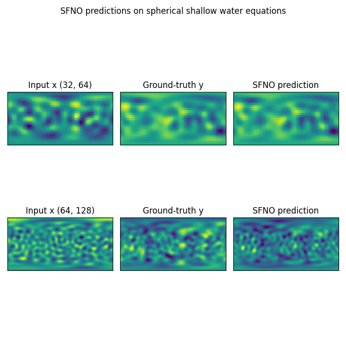
Visualizing SFNO predictions on spherical data
We visualize the model’s predictions on spherical shallow water equations data. Note that we trained on a very small resolution for a very small number of epochs. In practice, we would train at larger resolution on many more samples.
However, for practicality, we created a minimal example that: i) fits in just a few MB of memory ii) can be trained quickly on CPU
In practice we would train a Neural Operator on one or multiple GPUs
fig = plt.figure(figsize=(7, 7))
for index, resolution in enumerate([(32, 64), (64, 128)]):
    test_samples = test_loaders[resolution].dataset
    data = test_samples[0]
    # Input x
    x = data['x']
    # Ground-truth
    y = data['y'][0, ...].numpy()
    # Model prediction: SFNO output
    x_in = x.unsqueeze(0).to(device)
    out = model(x_in).squeeze()[0, ...].detach().cpu().numpy()
    x = x[0, ...].detach().numpy()

    # Plot input fields
    ax = fig.add_subplot(2, 3, index*3 + 1)
    ax.imshow(x)
    ax.set_title(f'Input x {resolution}')
    plt.xticks([], [])
    plt.yticks([], [])

    # Plot ground-truth fields
    ax = fig.add_subplot(2, 3, index*3 + 2)
    ax.imshow(y)
    ax.set_title('Ground-truth y')
    plt.xticks([], [])
    plt.yticks([], [])

    # Plot model prediction
    ax = fig.add_subplot(2, 3, index*3 + 3)
    ax.imshow(out)
    ax.set_title('SFNO prediction')
    plt.xticks([], [])
    plt.yticks([], [])

fig.suptitle('SFNO predictions on spherical shallow water equations', y=0.98)
plt.tight_layout()
fig.show()
Total running time of the script: (1 minutes 22.537 seconds)